Abstract
Vortex electromagnetic waves have superior performance over electromagnetic waves. In order to improve the radar super-resolution lateralization technique in its missing modes, this study proposes to start from the perspective of mode missing. The missing modes are reconstructed using the Adaptive Step Size Gradient Descent (ASSGD) method by exploiting the features of the missing modes. The linear minimum mean square error (LMMSE) estimation method is also used to solve the problem of poor reconstruction accuracy due to the Missing Modes. The Missing Modes Iterative Adaptive Approach (MMIAA) algorithm and Missing Modes Sparse Learning via Iterative Minimization (MMSLIM) algorithm are then used. Minimization (MMSLIM) algorithm to recover missing modes. The results showed that the RMSEs of the recovery errors of MMSLIM, MMIAA and ASSGD were 0.16, 0.31 and 0.82 respectively at a modal missing ratio of 0.7, while ASSGD fails to recover the missing modal data at a modal missing ratio of 0.9. The overall data quality of the azimuthally estimated RMSE was average when the signal-to-noise ratio was at [–5, 10] dB. And the curve becomes flatter when it reaches 15 dB or more, indicating that MMSLIM, MMIAA has important theoretical and practical value.
1. Introduction
Due to the transmission characteristics of electromagnetic waves, radar has the characteristics of all-weather, all-day, long-distance work, it can obtain the scattering information of electromagnetic waves in a variety of complex environments, and achieve the detection, identification and tracking of targets, known as the “eyes” of modern information warfare [1]. In recent years, along with the continuous progress of radar detection technology, various types of radar have been widely used in all walks of life. It can achieve battlefield surveillance, target reconnaissance, guidance and anti-missile functions in the military, and in civilian use for terrain observation, automatic navigation, weather warning and many other fields. Vortex electromagnetic waves not only retain the frequency, phase and amplitude characteristics of conventional electromagnetic waves, but their spiral wavefront brings new degrees of freedom to signal modulation, allowing them to propagate multiple orthogonal and dissimilar wave arrays at the same time, thus achieving infinite propagation [2]. For this reason, it has been used in communications to increase the speed of communication. Its application to radar, however, is a fledgling technology that needs to be studied in depth. Vortex electromagnetic wave radar is able to obtain information about features in another dimension due to the vortex electromagnetic wave it emits in the radar exposure area, which not only produces a time-varying wavefront, but also a null-varying wavefront at its beam. It is therefore of great importance for high-precision guidance, three-dimensional detection in complex environments, three-dimensional imaging in the air, and super-resolution direction finding. Due to its Orbital Angular Momentum (OAM) property, the wavefront phase of vortex electromagnetic waves has a unique spiral shape and the number of modes is infinite orthogonal, which brings new space for electromagnetic wave propagation [3]. Vortex radar is a type of radar that uses vortices to achieve detection of multiple targets and can effectively overcome disadvantages such as the inability of real-aperture radar to effectively detect targets in waves. The vortex electromagnetic wave radar super-resolution direction finding technology, i.e. based on the phase difference of multiple modal number echoes of OAM, uses super-resolution algorithms such as spectral estimation and sparse recovery algorithms to achieve vortex radar orientation super-resolution under a small number of modal numbers and mode-deficient conditions. The innovation of this study lies in starting from the perspective of modal missing, utilizing the characteristics of modal missing, using adaptive step gradient descent method to reconstruct missing modes, and combining linear minimum mean square error estimation to solve the problem of low reconstruction accuracy caused by modal missing; And use iterative adaptive missing mode recovery algorithm and sparse loop iterative minimization missing mode recovery algorithm to recover missing modes.
2. Related works
Eddy electromagnetic wave radar has been widely used in various industries. Chen Y. et al. studied the Doppler and micro-Doppler effects for the wider application of eddy electromagnetic waves in target detection. The research results show that the vortex EM wave effect is more complex than non-vortex EM wave, and the former can provide more features for target identification [4]. Yuan H. et al. proposed a vortex EM wave radar-based algorithm for microwave parameter extraction of rotating targets with rough estimation of microwave parameters through linear Doppler, etc., in response to the problem that existing microwave extraction algorithms are less efficient in the presence of multiple scattering points. The experimental results show that the algorithm has a good performance [5]. Kim S. et al. proposed a super-resolution-based radar boda estimation method in order to improve the performance of radar waves and simulate the data between antennas using extrapolation for virtual ground generation. The results show that the method is less complex and close to the root mean square error of the conventional method [6]. Chen H. T. et al. conducted a study based on full-wave electromagnetic simulation and near-field diagnostic principles in order to investigate the near-field scattering characteristics of typical scatterers under vortex electromagnetic wave irradiation. The results showed that vortex electromagnetic waves have a high ability to identify the characteristics of scatterers [7].
Guo S. et al. proposed a mechanically controlled imaging high-resolution imaging method based on electromagnetic vortex beam imaging in order to improve the high resolution of the imaging. The results showed that the method can reduce the number of orbital angular momentum modes and improve the imaging resolution [8]. Yuan H. et al. proposed a high-resolution imaging method based on a uniform circular array antenna for the problem of low quality of uniform circular array imaging. and in the process, the echoes are not dependent on the vortex electromagnetic waves. The experimental data verified that the method would improve the imaging resolution [9]. Wang Y. et al. established a Doppler detection model for radar systems based on orbital angular momentum by using vortex electromagnetic waves with multiple orbital angular momentum to detect rotating objects at arbitrary positions. Simulation results show that the model has certain validity and can obtain more detailed rotation parameters [10]. Lin Y C et al. proposed a low-complexity high-resolution BODA method in order to improve the allocation rate of sparse multi-input multi-output radar. Simulation results show that the method has some validity and is able to reduce the complexity while increasing the resolution [11].
The above results show that the vortex EM wave radar has good applications, but its performance needs to be improved. In view of this, the study will recover its missing modes to improve the lateral performance of the radar super-resolution.
3. Super-resolution direction finding for missing mode recovery in vortex electromagnetic wave radar
3.1. Super-resolution direction finding technique for vortex electromagnetic wave radar based on ASSGD missing mode recovery
For some modes of vortex waves, the scattered echoes from the scattered body under test are attenuated, resulting in the phenomenon of missing modes. When the modes are missing, the super-resolution method suffers from reduced resolution, increased partials and increased peak partials, which in turn reduces the azimuth spectrum resolution and prevents a clear image of the target from being obtained. Due to the missing modes, the azimuth spectrum imaging quality of the radar is significantly degraded. How to improve the super-resolution capability of the vortex EM wave radar under missing modes is an urgent problem to be solved.
When a vortex electromagnetic wave radar operates, the modes are received in sequence, with the power value of their background noise as the recognition threshold. During reception, the energy share of the mode is counted and if the energy level of the dominant mode is lower than the background noise, the mode is considered not to have been received correctly, i.e. the mode is missing. When the target is at rest, the vortex radar echo is seen as a superposition of signals from multiple targets, such that both the valid and missing modes acquired by the vortex radar have the same azimuthal spectral component. The missing modes can then be recovered from these valid modes to obtain better azimuthal spectral results.
Assuming that there are samples of received modes, if there is a case where the primary mode energy of a received mode exceeds the discrimination threshold, it is included in , where, , is used to describe the set of samples of consistently normally received modes [12]. Conversely, if a situation arises where the received modal major mode energy is below the discrimination threshold, it is included in , the set of samples of missing modes, and a sketch of the sampling segments for valid and missing modes is shown in Fig. 1.
Fig. 1Sampling section diagram of effective mode and missing mode
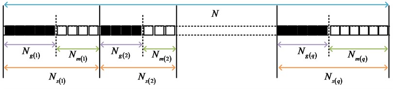
In Fig. 1, the received modal samples are divided into a valid modal subset and a missing modal subset . the and are represented using a matrix with the expression shown in Eq. (1):
In Eq. (1), and are used to describe the data matrix in the normal reception mode and the missing mode, then is meant to be the data of all the modes that should be received [13].
In response to the current situation of missing modes in the OAM modal data acquired by the vortex radar, the use of existing super-resolution methods will result in low resolution and the inability to perform high partials, so in order to estimate the vortex radar azimuth spectrum more accurately, the missing mode sample needs to be estimated in .
The gradient descent algorithm (GDA) is based on the sparsity of the target along the azimuthal spectrum, with the sparsity of the signal as the optimisation objective. Usually, the azimuthal spectral parametrization decreases exponentially and can be considered as 0 when it is below a certain threshold, while when it is above the threshold, the amount is the sparsity of the signal. The ideal fully sampled modal sample would result in a very low azimuthal spectral sparsity, while a modal deficiency would result in an increase in azimuthal spectral sparsity, which could be raised to the optimisation objective. The Adaptive Step Size Gradient Descent (ASSGD) algorithm can adaptively adjust the step size within each gradient descent cycle, thus improving the convergence and accuracy of the algorithm.
When the number of targets is smaller than the number of signal samples, the signal is considered to be sparse in the orientation domain. A sparse signal is able to be recovered from a small number of sample signals by a full signal. In practice, when the signal is represented as sparse in the transform domain, the sampled data is usually used as the observed data. gda uses the lost sample signal as a variable, and the complete signal is diluted in the transform domain, i.e. the degree of sparsity obtained is reduced, by modifying the corresponding rule at each iteration for the lost sample data [14].
For missing modal data, GDA treats its normally received modal signal value as a constant and treats the sampled value of the missing modal signal as a continuous variable. Denote the sparsity of the signal by , where is used to describe the matrix parametrization, and then represents the linear transform, which is generally obtained by the discrete Fourier transform of the signal , or .
Firstly, the initial signal will represent the data of the full pattern received, where the missing data will be given an initial value of 0, and the initial iterative signal will be defined with the expression shown in Eq. (2):
where is used to describe the first iteration of the algorithm [15]. Then, regarding the missing mode at , two signals, and , are formed at the th iteration, and the expression for is shown in Eq. (3):
where, , and is a constant, which is used to determine whether the step size of the missing modal signal sample value should be increased or decreased during each iteration. Similarly, the expression for is shown in Eq. (4):
Then, the difference of the gradient vector is estimated, where the coordinate of this gradient vector is considered as a constant when it is on a normal sample of the received modal signal, so the value of the coordinate of this gradient vector is 0. Conversely, if the coordinate of the gradient vector is positioned on the sample point of the missing modal signal, it is solved as the difference of the signal sparsity. Then, during the th iteration, the coordinates of the gradient vector are shown in Eq. (5):
And the value of the signal is corrected by the gradient vector during the continuous iteration, the expression is shown in Eq. (6):
where, is used to describe the difference step at each iteration and is assigned the value . Iteratively, the above steps are performed and the missing modal sampling values eventually converge to a sampling point in the modal domain with minimum sparsity; meanwhile, the performance of the algorithm depends on the parameter .
When a sample point is a missing modal sample signal, the sparsity of the sample point varies with increasing step or decreasing step of the signal at the sample point [16]. Assuming that the exact value of the missing mode has been obtained, the form of the sparse signal in the modal domain can be expressed as Eq. (7):
Since the gradient vector is estimated using the difference of sparsity, the gradient with -paradigm is constant under conditions close to the optimality of the algorithm, so it cannot be solved with more accuracy than the step size . Then when the initial step size is too large, the method is not accurate enough. If the initial step size is small, it leads to a large number of iterations, which results in inefficiency and wasted time. The best approach is the adaptive step size approach, where the step size is increased when the sparsity does not converge to a minimal point. The step size is reduced when the sparsity converges to a minima. That is, GDA recovers the missing modes as shown in Fig. 2.
Fig. 2GDA restoration process of missing modes
3.2. Vortex electromagnetic wave radar super-resolution direction finding technique based on LMMSE for missing mode recovery
The results of GDA-based missing mode recovery are affected by the number of valid modes obtained, and if the number of obtained modes is small, the recovery results will be worse. In view of this, the study will recover the missing modes based on Linear minimum mean square error (LMMSE). First, a preliminary spectral estimation is performed based on the obtained effective modal data vector to obtain a coarse spectrum. Then, a linear relationship between the effective and missing mode vectors is derived. Finally, the linear transformation of the valid modes is used to estimate the missing modes.
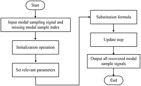
Two methods, IAA and SLIM, are used to obtain better orientation spectra with less OAM. On this basis, coarse spectral estimation is performed using these two methods, followed by linear estimation. This leads to modal recovery algorithms called Missing Modes Iterative Adaptive Apporoach (MMIAA) based algorithm, Missing Modes Sparse Learning via Iterative Minimization (MMSLIM) algorithm. In particular, the process of the MMIAA recovery algorithm is shown in Fig. 3.
Fig. 3Process of MMIAA recovery algorithm
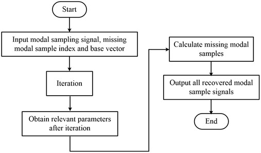
As can be seen in Fig. 3, the iterative process needs to be repeated in the MMIAA recovery algorithm until the algorithm converges. Similarly, the process of the MMSLIM recovery algorithm is similar to Fig. 3.
To estimate the coarse spectrum using IAA in the effective mode, the azimuthal domain needs to be first decomposed into equally spaced grid points, assuming , and that is the target scattering coefficient corresponding to that point in this azimuthal domain; usually, will take a larger value to obtain better azimuthal resolution [17]. Where the complete modal domain signal expression is shown in Eq. (8):
where, is the target scattering coefficient and is meant to be the noise signal at the different modes [18]. The initial spectral estimation of the modal data can generally be performed using weighted least squares, then the spectral estimation at is able to be converted to Eq. (9):
Solving for the partial derivatives of enables a weighted least squares estimate to be obtained, with the expression shown in Eq. (10):
By means of matrix inverse derivation, it is possible to obtain the Eq. (11):
Considering that all meshes require repeated calculations for , to circumvent this phenomenon, Eq. (11) is substituted into Eq. (10) so that the number of times needs to calculate the matrix inverse during each iteration is only one; and the expression for each iteration of is obtained, as shown in Eq. (12):
Because the complex amplitude at each grid point must be known in order to perform the calculation of , the can be assigned as a unit matrix when the initialization is performed. During subsequent iterations, the estimated in the previous iteration is used continuously to calculate . If the difference between the results obtained from two adjacent iterations is below a certain threshold, then the iteration is terminated [19].
Once the coarse spectrum has been estimated from the obtained modal data, the missing modal data can be recovered from the coarse spectrum, i.e. by linear transformation of . The expression is shown in Eq. (13):
Therefore, it is possible to estimate using linear minimization of mean square error, and the expression of mean square error of is shown in Eq. (14):
The equality sign in Eq. (14) can hold when . Then the root mean square error of can be optimally estimated at this time, and the expression is shown in Eq. (15):
Eq. (15) shows that when the posterior is calculated, can be found, and then multiplied with the numerator of the iterative equation, can be calculated [20].
4. Analysis of missing mode recovery results under vortex electromagnetic wave-based radar super-resolution lateralization technique
4.1. Simulation results of missing mode recovery based on ASSGD and LMMSE
Firstly, the missing mode recovery results based on ASSGD are analysed, and the missing modes are recovered using the gradient descent method, and simulation experiments are carried out. The computer system used in the experiment was Windows 8, and the programming tool was Python. The parameters of the simulation include: 10 GHz vortex EM signal frequency, 4 UCA array element diameter, the number of emitted OAM modes set to [–25, 25], a total of 50 OAM modes, and a signal-to-noise ratio of 15 dB. The original signal is generated by setting two ideal object scattering points on 50 and 70. Of the 50 modes, 20 were lost randomly, i.e., the mode-missing ratio was 40 %. Generally, with missing modes, there are many zero values in the received signal and the gradient descent method to recover the missing modes is shown in Fig. 4.
The experimental results show that GDA is able to recover the sample values of the missing modes very well. Their orientation spectra were obtained by performing FFT calculations on the original fully modal sample signal, the received signal in the missing mode, and the sample signal after recovering the mode, respectively. The results are shown specifically in Fig. 5.
Fig. 4Comparison of sample values of restored mode and original mode
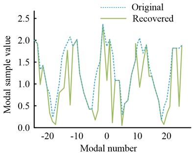
a) All modal samples
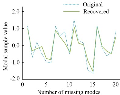
b) Missing modal samples
Fig. 5Normalized azimuth spectrum of sample signal under three modes
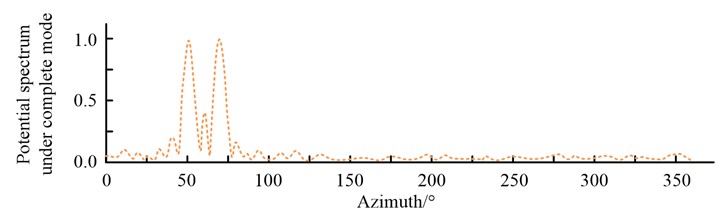
a) Normalized azimuth spectrum of sample signal in complete mode
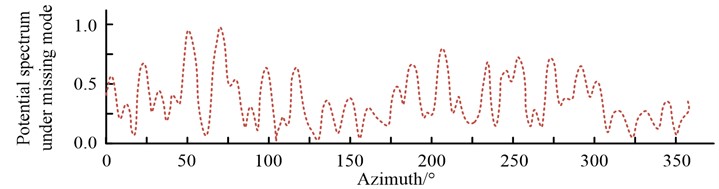
b) Normalized azimuth spectrum of sample signal in missing mode
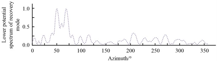
c) Normalized azimuth spectrum of sample signal under recovery mode
Fig. 5 shows that the missing mode significantly affects the azimuthal spectrum, increasing the number of partials in the azimuthal spectrum significantly, and if the missing mode is restored, the effect of the partials is somewhat diminished.
The LMMSE-based missing modes are then simulated and analysed by first generating the vortex radar echoes of the missing modes and simulating them. The parameter settings during the simulation are the same as in Section 1, and out of 50 modes, 25 modes are lost randomly, i.e., the mode missing ratio is 50 %. At the same time, the number of missing modes, the original signal and the actual received signal with the missing modal data are significantly different. Using the MMIAA and MMSLIM algorithms, the sample data of the received missing modal signal was recovered and the results are shown in Fig. 6.
Fig. 6Comparison of restored mode and original mode sample values by two methods
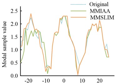
a) All modal samples data
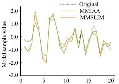
b) Missing modal samples will restore sample data
Fig. 7Normalized azimuth spectrum of sample signal in four cases
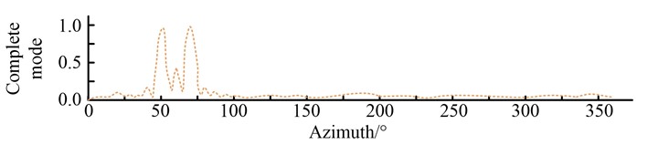
a) Normalized azimuth spectrum of sample signal in complete mode
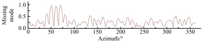
b) Normalized azimuth spectrum of sample signal in missing mode
c) Normalized azimuth spectrum of sample signal under recovery mode
d) Normalized azimuth spectrum of sample signal under recovery mode
As can clearly be observed in Fig. 6, both methods recover the sample values of the missing modes very well at a modal deficiency rate of 50 %. And the MMSLIM algorithm outperforms the MMIAA algorithm in that the former recovers the sample values of the modes that are essentially identical to the values of the original signal.
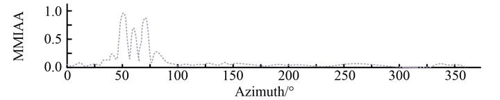
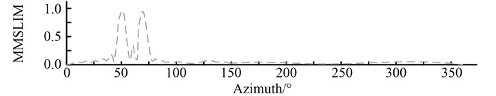
The orientation spectrum of the original fully modal sample signal, the received signal in the missing mode, the modal sample signal after MMIAA recovery, and the modal signal after MMSLIM recovery were solved using the FFT method, and the results are shown in Fig. 7.
It can be found that the missing mode has a significant effect on the formation of the azimuthal spectrum. After the missing modes were recovered using MMIAA and MMSLIM, the side flaps of the azimuthal spectrum were significantly reduced compared to the missing modes, and the resulting azimuthal spectrum was basically the same as that of the full modal sample.
4.2. Algorithm performance analysis
Simulation experiments of the three algorithms under study are carried out for snail-rotation radar in a mode-deficient environment. The differences in the experimental results of the three algorithms under different simulation conditions are evaluated using metrics such as root mean square error of recovery accuracy, root mean square error of spectral estimation super-resolution after recovering the modalities, and combined with Monte Carlo random experiments to estimate RMSE and RMSE of recovery accuracy.
Simulation tests were carried out for ASSGD, MMIAA and MMSLIM to compare the effectiveness of the three methods in the case of modal deficiencies. The root-mean-square error of recovery accuracy, the root-mean-square error metric of super-resolution of spectral estimation after recovering the modalities are used for evaluation, and the RMSE and RMSE of recovery accuracy are estimated in conjunction with Monte Carlo random experiments.
First, the recovery accuracy of the ASSGD, MMIAA and MMSLIM algorithms is compared for different modal deficit ratios. The main simulation parameters are set in the same way as in Section 1. Also, from the 50 modes, a specific proportion of modes is selected and simulated for the case of missing modes. The modal missing ratios were set to 0-0.9, and the number of Monte Carlo experiments at all missing ratios was 100. The missing modes were also recovered using three algorithms and RMSE analysis was performed on the results recovered by the three algorithms and the results are shown in Fig. 8.
Fig. 8Recovery error of three algorithms under different modal loss ratios
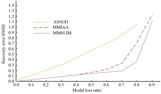
Fig. 8 gives the missing ratios of the three methods for various modal missing ratios. It can be seen that the recovery accuracy of all three methods decreases as the modal missing ratio increases. In the case of obtaining the full modal sample, no recovery is required and the error is 0. The high recovery accuracy of MMSLIM is MMSLIM, MMIAA and ASSGD in descending order. at a modal missing ratio of 0.7, the recovery error RMSE for MMSLIM, MMIAA and ASSGD are 0.16, 0.31 and 0.82 respectively. while at a model missing ratio of 0.9, ASSGD was unable to recover the missing modal data.
Based on this, the study proposes to use three modal recovery methods. The vortex radar azimuth spectrum is calculated using the radar echo data under modal deficiency and the echo data after modal recovery, respectively. The mathematical model of the vortex radar azimuth spectrum is also established using the RMSE of the azimuth angle to the original target as the evaluation criterion. To address the problem that the accuracy of the above method will drop significantly after the modal loss ratio reaches 0.7, the study set the modal loss ratio between 0 and 0.7, 100 Monte Carlo random trials, each round of experiments set two random targets with azimuth interval of 10, the signal-to-noise ratio is 15dB, the simulation results are shown in Fig. 9.
Fig. 9Estimated RMSE of target orientation after modal restoration by three algorithms under different modal loss ratios
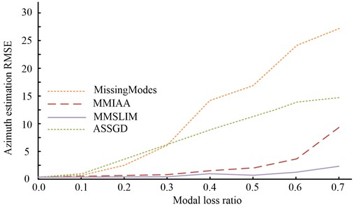
In Fig. 9, it can be seen that the modal loss has a significant impact on the directional accuracy of the vortex radar, while the recovered directional accuracy is improved to some extent by using various modal recovery methods. The difference between the directional accuracy recovered by the MMSLIM method and that recovered by the MMSLIM method is not significant. The recovery accuracies of the three algorithms were then calculated for different signal-to-noise ratios. The aim of this experiment is to evaluate the RMSE of the various methods for vortex radar recovery at different S/N ratios. the total number of OAM modes is set to 50, the modal loss ratio is set to 0.7, the S/N ratio is increased by 5 dB for every 5 dB from –5 to 30 dB, and the number of Monte Carlo experiments at each S/N ratio is 100.
Fig. 10Recovery RMSE of three algorithms under different SNR
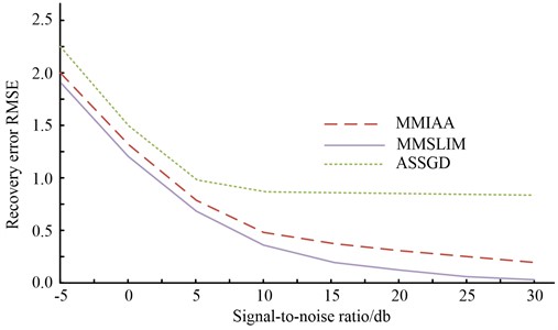
The simulation results are shown in Fig. 10, where, overall, the recovery error of each method decreases as the signal-to-noise ratio increases, and its accuracy improves. Furthermore, when the modal missing ratio is 0.7, each method can recover the missing modes at different levels, with the MMSLIM algorithm having the best results. Similar to the above simulation tests, the accuracy of the target orientation estimation after modal recovery was simulated by setting the modal missing ratio to 0.7 at –5 to 30 dB. The Monte Carlo tests were repeated 100 times for different signal-to-noise ratios, with randomised azimuths for each test subject.
Fig. 11Estimation of target bearing RMSE after modal recovery under different signal-to-noise ratios
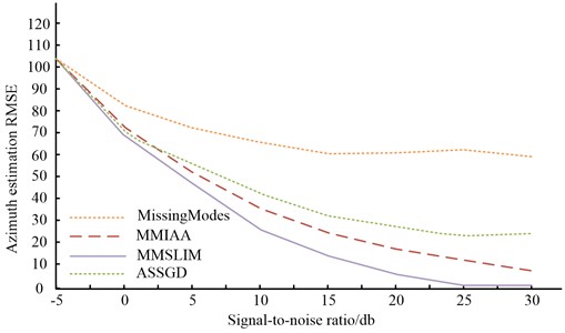
From the simulation results in Fig. 11, it can be seen that the accuracy of the azimuth estimation continues to increase as the signal-to-noise ratio continues to increase, but the RMSE through modal recovery is better than the accuracy in the missing modal case. When the S/N ratio is at [–5, 10] dB, the overall data quality is average. And at reaching 15 dB or more, the conditions of the algorithm can be met and the curve becomes smoother. The accuracy of the three algorithms was analyzed, and the results are shown in Fig. 12.
Fig. 12Accuracy analysis of three algorithms
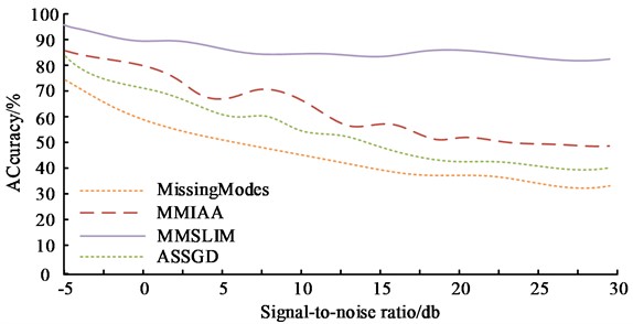
From Fig. 12, it can be seen that as the signal-to-noise ratio continues to increase, the prediction accuracy of the three algorithms decreases. However, overall, the prediction accuracy of the three algorithms is MMSLIM, MMIAA, and ASSGD from high to low.
Table 1Analysis results of three algorithms
Number | Project | MMSLIM | MMIAA | ASSGD |
(1) | Modal missing ratio 0.7 | 0.16 | 0.31 | 0.82 |
(2) | Recovery error under different signal-to-noise ratios | 0.1 | 0.2 | 0.8 |
(3) | Accuracy of azimuth estimation | 18 | 19 | 20 |
The results of the above simulations show that the three algorithms are in the order of MMSLIM, MMIAA and ASSGD in terms of the recovery accuracy of the missing modes, the accuracy of the recovered azimuth resolution and the complexity of the algorithm, while the results of the three algorithms are in the order of ASSGD, MMIAA and MMSLIM in terms of the recovered azimuth spectral parametrization level.
The analysis results of the three algorithms are shown in Table 1.
5. Conclusions
Eddy electromagnetic waves can improve the spectrum utilisation of a communication system and can also increase the channel capacity of the system. However, in real situations, the scattered signal between some modes of the vortex wave and the object under test is attenuated, resulting in a missing signal mode. This in turn reduces the azimuthal spectral resolution and prevents a high-resolution image of the target from being obtained. In view of this, a missing mode recovery algorithm based on LMMSE theory is proposed. Firstly, the scenario of missing modalities in a vortex radar is investigated and the missing modal is recovered based on the adaptive step GDA. It is demonstrated experimentally that the method proposed in the study can obtain good recovery results when the modal loss is small. Afterwards, the LMMSE method is used to transform the missing modes into a linear relationship between the effective modes, and the LMMSE method is used to achieve a fast estimation of the missing modes, and the recovery accuracy of the various methods is analysed and compared. It is experimentally verified that the proposed method outperforms the vortex radar in terms of orientation resolution capability when the modes are missing. At the same time, the number of required modes is reduced by using the OAM mode selection, thus reducing the computational complexity of the vortex radar and providing some guidance for the development of azimuthal super-resolution techniques for vortex radar. the recovery accuracy of ASSGD, MMIAA and MMSLIM all decrease with the increase of the mode-missing ratio, and the accuracy of all three decreases significantly after the mode-missing ratio reaches 0.7. When the modal missing ratio is 0.7, each method can recover the missing modes at different levels, and the MMSLIM algorithm has the best results. However, all targets set in this experiment are ideal point targets, and further research is needed to include scene reconstruction of complex targets.
References
-
Z. Zhou, Y. Wang, J. Yu, W. Guo, and Z. Li, “Super-resolution reconstruction of plane-wave ultrasound image based on a multi-angle parallel u-net with maxout unit and novel loss function,” Journal of Medical Imaging and Health Informatics, Vol. 9, No. 1, pp. 109–118, Jan. 2019, https://doi.org/10.1166/jmihi.2019.2548
-
H. Lee, J. Kim, and J. Choi, “A compact Rx antenna integration for 3D direction-finding passive radar,” Journal of Electromagnetic Engineering and Science, Vol. 19, No. 3, pp. 188–196, Jul. 2019, https://doi.org/10.26866/jees.2019.19.3.188
-
A. N. Abdullah, L., and Ali, “Comparative study of super-performance DOA algorithms based for RF source direction finding and tracking,” Technology Reports of Kansai University, 2021.
-
Y. Luo, Y.J. Chen, Y.Z. Zhu, W.Y. Li, and Q. Zhang, “Doppler effect and micro‐Doppler effect of vortex‐electromagnetic‐wave‐based radar,” IET Radar, Sonar and Navigation, Vol. 14, No. 1, pp. 2–9, Jan. 2020, https://doi.org/10.1049/iet-rsn.2019.0124
-
H. Yuan, Y. Luo, Y. J. Chen, J. Liang, and Y.X. Liu, “Micro‐motion parameter extraction of rotating target based on vortex electromagnetic wave radar,” IET Radar, Sonar and Navigation, Vol. 15, No. 12, pp. 1594–1606, Dec. 2021, https://doi.org/10.1049/rsn2.12149
-
S. Kim, B. Kim, Y. Jin, and J. Lee, “Super-resolution-based DOA estimation with wide array distance and extrapolation for vital FMCW radar,” Journal of Electromagnetic Engineering and Science, Vol. 21, No. 1, pp. 23–34, Jan. 2021, https://doi.org/10.26866/jees.2021.21.1.23
-
Hai-Tao Chen, Ze-Qi Zhang, and Jie Yu, “Near-field scattering of typical targets illuminated by vortex electromagnetic waves,” Applied Computational Electromagnetics Society Journal, Vol. 35, No. 2, pp. 129–134, 2020.
-
S. Guo, Z. He, Z. Fan, and R. Chen, “High‐resolution passive imaging by electromagnetic vortex beams,” Microwave and Optical Technology Letters, Vol. 64, No. 1, pp. 97–103, Jan. 2022, https://doi.org/10.1002/mop.33056
-
H. Yuan, Y.-J. Chen, Y. Luo, J. Liang, and Z.-H. Wang, “A resolution-improved imaging algorithm based on uniform circular array,” IEEE Antennas and Wireless Propagation Letters, Vol. 21, No. 3, pp. 461–465, Mar. 2022, https://doi.org/10.1109/lawp.2021.3135806
-
Y. Wang, K. Liu, H. Liu, J. Wang, and Y. Cheng, “Detection of rotational object in arbitrary position using vortex electromagnetic waves,” IEEE Sensors Journal, Vol. 21, No. 4, pp. 4989–4994, Feb. 2021, https://doi.org/10.1109/jsen.2020.3032665
-
Y.-C. Lin and T.-S. Lee, “max-MUSIC: a low-complexity high-resolution direction finding method for sparse mimo radars,” IEEE Sensors Journal, Vol. 20, No. 24, pp. 14914–14923, Dec. 2020, https://doi.org/10.1109/jsen.2020.3009426
-
X. Sun, J. Shao, B. Dan, and Q. Li, “A novel multi-modal OAM vortex electromagnetic wave microstrip array antenna,” Journal of Communications and Information Networks, Vol. 4, No. 4, pp. 95–106, 2019.
-
H. Liu, Y. Wang, J. Wang, K. Liu, and H. Wang, “Electromagnetic vortex enhanced imaging using fractional OAM beams,” IEEE Antennas and Wireless Propagation Letters, Vol. 20, No. 6, pp. 948–952, Jun. 2021, https://doi.org/10.1109/lawp.2021.3067914
-
A. M. Zheltikov, “State-vector geometry and guided-wave physics behind optical super-resolution,” Optics Letters, Vol. 47, No. 7, pp. 1586–1589, Apr. 2022, https://doi.org/10.1364/ol.441643
-
X. Tuo, Y. Zhang, Y. Huang, and J. Yang, “Fast sparse-TSVD super-resolution method of real aperture radar forward-looking imaging,” IEEE Transactions on Geoscience and Remote Sensing, Vol. 59, No. 8, pp. 6609–6620, Aug. 2021, https://doi.org/10.1109/tgrs.2020.3027053
-
Q. Zhang et al., “TV-sparse super-resolution method for radar forward-looking imaging,” IEEE Transactions on Geoscience and Remote Sensing, Vol. 58, No. 9, pp. 6534–6549, Sep. 2020, https://doi.org/10.1109/tgrs.2020.2977719
-
Y. Li, J. Liu, X. Jiang, and X. Huang, “Angular superresol for signal model in coherent scanning radars,” IEEE Transactions on Aerospace and Electronic Systems, Vol. 55, No. 6, pp. 3103–3116, Dec. 2019, https://doi.org/10.1109/taes.2019.2900133
-
G. Yang, Y. Liu, Y. Yan, and W. Li, “Vortex wave generation using single‐fed circular patch antenna with arc segment,” Microwave and Optical Technology Letters, Vol. 63, No. 6, pp. 1732–1738, Jun. 2021, https://doi.org/10.1002/mop.32806
-
J. Guo, H. Shi, T. Yang, C. Lv, and Z. Qiao, “Atmospheric turbulence compensation for OAM-carrying vortex waves based on convolutional neural network,” Advances in Space Research, Vol. 69, No. 5, pp. 1949–1959, Mar. 2022, https://doi.org/10.1016/j.asr.2021.11.039
-
F. Shen, J. Mu, K. Guo, and Z. Guo, “Generating circularly polarized vortex electromagnetic waves by the conical conformal patch antenna,” IEEE Transactions on Antennas and Propagation, Vol. 67, No. 9, pp. 5763–5771, Sep. 2019, https://doi.org/10.1109/tap.2019.2922545
About this article

The authors have not disclosed any funding.
The datasets generated during and/or analyzed during the current study are available from the corresponding author on reasonable request.
The authors declare that they have no conflict of interest.
