Application of machine learning algorithms in drug screening

Jin, Ke; Rong, Cunqing; Chang, Jincai

doi:10.21595/chs.2023.23292

Journal of Complexity in Health Sciences

Browse Journal

Submit article

Published: 04 November 2023

Check for updates

Application of machine learning algorithms in drug screening

Ke Jin¹

Cunqing Rong²

Jincai Chang³

^{1, 2}College of Sciences, North China University of Science and Technology, Tangshan, 063210, China

³3D Modeling and Application Innovation Laboratory, North China University of Science and Technology, Tangshan, 063210, China

Corresponding Author:

Jincai Chang

Cite the article Download PDF

Downloads 62

Abstract

At present, in the medical field, drug screening is usually performed using in vivo drug experiments. However, it is very time-consuming and laborious to conduct in vivo experiments on a large number of drugs to be screened one by one. This paper attempts to propose using machine learning algorithms to perform preliminary screening of a large number of compounds to be screened and their molecular structures to reduce the workload of in vivo experiments. Among them, it is internationally recognized that there is an important association between breast cancer progression and the alpha subtype of the estrogen receptor. Anti-breast cancer drug candidates with excellent efficacy need to contain compounds that can better antagonize ERα activity. In this paper, the research object is narrowed down from compounds to the molecular structure of the compounds, and then the random forest regression algorithm is used to develop the molecular structure-ERα activity prediction model. Molecular structures with significant effects on biological activity were screened from molecular structure descriptors in numerous compounds. Four different kernel functions were used to conduct comparative experiments, and finally a support vector regression algorithm based on radial basis kernel function was established, which realized the quantitative prediction of compounds on biological activity of ERα, and could find potential compounds beneficial to breast cancer treatment. This is a novel, computer-based method for preliminary drug screening, which can help medical researchers effectively narrow the scope of experiments and achieve more accurate optimization of drugs.

Application of machine learning algorithms in drug screening

Highlights

Propose the use of machine learning algorithms for preliminary screening of a large number of compounds and molecular structures to reduce the workload of in vivo experiments.
Reduce the research object from compounds to the molecular structures that make up the compounds, and screen out molecular structures that have a significant impact on biological activity from the molecular structure descriptors of numerous compounds.
Four different kernel functions were used for comparative experiments, and a support vector regression algorithm based on radial basis kernel functions was ultimately established. This algorithm achieved the effect of compounds on ER α Quantitative prediction of biological activity can find potential compounds beneficial to breast cancer treatment.

1. Introduction

In recent years, with the accelerated pace of people’s lives, external factors such as smoking, alcoholism and poor eating habits lead to an increasing risk of breast cancer. Breast cancer is known as the number one killer that threatens women’s health. According to the “Global Cancer Statistics 2020” jointly released by the World Health Organization (WHO), the International Agency for Research on Cancer (IARC) and the Cancer Society (ACS) in 2020, the incidence of breast cancer is increasing rapidly, accounting for 11.7 % of all cancer cases. Breast cancer, with 2.26 million cases worldwide, has surpassed lung cancer with 2.2 million cases to become the number one cancer in the world, and the number of cases of breast cancer is higher in developing countries [1]. Anticancer treatment has always been an important problem in medicine, but good development and progress have been made in the detection and precise treatment of breast cancer [2]. If timely detection and active treatment are available, most breast cancer patients have a higher probability of survival than other cancer patients. Under the current level of medical care, the 5-year survival rate of breast cancer patients can reach more than 89 %. Such good therapeutic effect of breast cancer is mainly attributed to the emergence of a large number of estrogen receptor (ERα) antagonist drugs in recent years, such as tamoxifen and raloxifene [3], the most commonly used drugs in the clinical treatment of breast cancer.

ERα is a regulatory protein that can interact with different agonists and antagonists, as well as transcriptional activators and inhibitors to undergo extensive remodeling [4]. Estrogen receptors do have an important impact on the development of breast cancer [5]. Estrogen receptors alpha (ERα) is expressed in 50 %-80 % of breast tumor cells, while the probability of expression in normal breast epithelial cells is no more than 10 %. Antihormone therapy is now used to treat patients with ERα-expressing breast cancer by regulating estrogen receptor activity to further controls estrogen levels in the body. Therefore, ERα is now recognized by the medical community as an important target for breast cancer treatment [6]. Drugs containing compounds that are better antagonistic to ERα activity are more suitable as anti-breast cancer drug candidates. For example, Wang Qiang demonstrated that tamoxifen and 17-β Estradiol can interact with ERα. The combination of 36 reveals ERα 36 mediates the molecular mechanism of tamoxifen in promoting breast cancer metastasis, which provides an important basis for molecular typing and individualized treatment of breast cancer [7]. However, there may be thousands of compounds that affect the biological activity of ERα. It will consume a lot of time and cost to carry out pharmaceutical experiments for each compound. Moreover, each compound contains nearly a thousand molecular structures, and not all molecular structures contained in a compound have an effect on the biological activity of ERα, so it is inappropriate to establish a direct mapping relationship between the compounds and the biological activity of ERα.

Recently, data mining methods such as data analysis and machine learning have also been gradually applied to predict ERα biological activity and screen related drugs. In 2022, Du Xueping proposed the use of multiple linear regression models to establish compounds for predicting ERα activity, proving the feasibility of using data analysis methods to predict ERα activity, providing great inspiration [8]. In the same year, He Yi and others used 3 σ. After the Outlier are removed from the criteria, the Random forest algorithm is used to predict the ERα biological activity, and a better prediction effect is obtained [9]. However, these models are all based on direct prediction of all compounds in the full dataset, and the high prediction accuracy was not achieved. In response to this issue, this article proposes a method to establish a model by first screening important compounds and then predicting their activity.

2. Data overview and preprocessing

2.1. Data overview

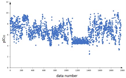
A total of 1974 compounds with bioactivity data against ERα are included in the dataset. Among them, the structural formulas of the 1974 compounds are provided, expressed as one-dimensional linear expressions SMILES (Simplified Molecular Input Line Entry System); The bioactivity of the compound against ERα is expressed as pIC₅₀ (IC₅₀ is an experimentally measured value in nM, the smaller the value the greater the bioactivity and the more effective it is in inhibiting ERα activity. The pIC₅₀ is the negative logarithm of the IC₅₀ value, which usually has a positive correlation with the bioactivity, i.e. a higher pIC₅₀ value indicates higher bioactivity). The 1974 compounds are numbered sequentially and the corresponding pIC₅₀ values are observed. The scatter diagram is shown in Fig. 1.

Based on the data characteristics it is found that there are no missing values in the data of 729 molecular descriptors constituting 1974 compounds, and the corresponding pIC₅₀ values are distributed in [2, 10] range. The distribution is overall uniform, with the pIC₅₀ values of the data numbered 1100 to 1300 concentrated on the [4, 5] range.

2.2. Data pre-processing

There is a dimension gap between the independent variables, which requires normalization of the data for easier application of subsequent data and to improve the accuracy of subsequent predictions [10]. Data normalization is to realize the indexation of statistical data. It mainly includes data trending processing and dimensionless processing. Data trending processing mainly solves the problem of data having different properties. The direct aggregation of indicators with different properties often does not correctly reflect the combined results of different influencing factors. We should first consider changing the nature of the inverse index data so that the forces of all indicators on the evaluation scheme are trended, and then aggregated to get the correct results. The dimensionless data processing mainly addresses the comparability of data. After the above standardization process, the original data are transformed into dimensionless index evaluation values, i.e., all index values are at the same quantitative level and can be comprehensively evaluated and analyzed. According to the distribution of the data set described in the previous subsection, the Min-max method is chosen here for normalization, and the specific formula is as follows:

1

x^{*} = \frac{x - m i n}{\max - m i n},

where $x$ denotes the original data, $x^{*}$ denotes the normalized data, min and max denote the minimum and maximum values of a certain group of data, respectively. After normalization, the data are mapped to the range of [0, 1] proportionally, and the indicators are in the same order of magnitude, which is convenient for subsequent use. The data normalization not only improves the convergence speed of the model, but also is helpful for the improvement of the classification accuracy and the computational accuracy of the model.

Fig. 1Distribution of plC50 values

3. Random forest-based molecular structure descriptor screening

3.1. Experimental process

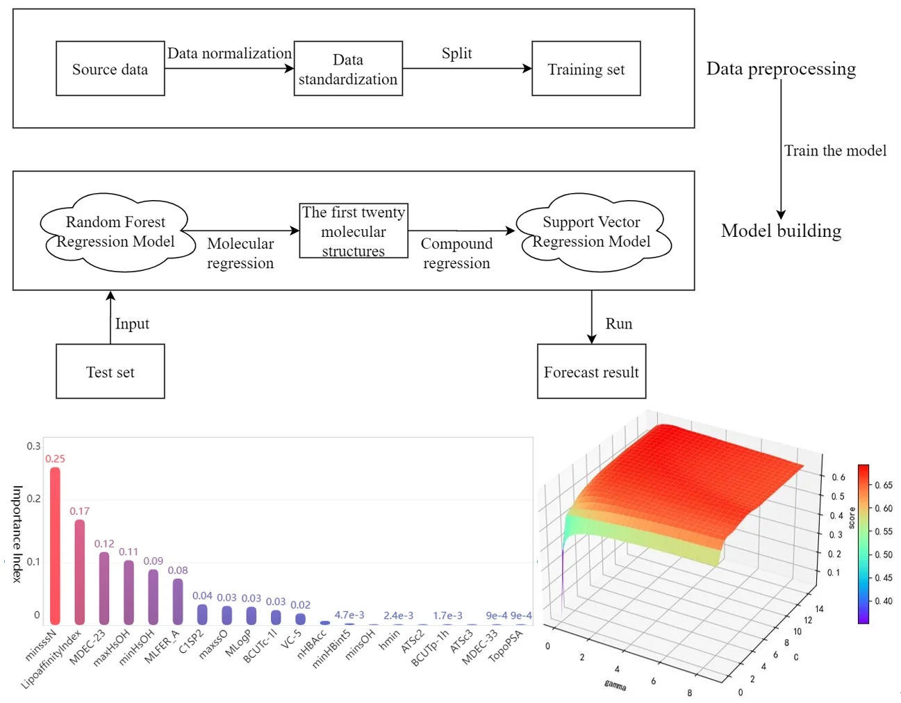
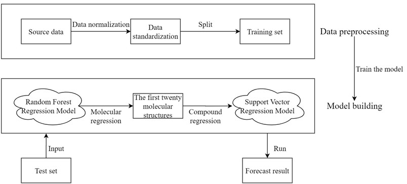
Before drug research and development, we can choose to establish the quantitative prediction model of each molecular structure in the compound to ERα biological activity to screen the compounds. The molecular structure descriptors are used to represent the corresponding molecular structures. The molecular structure descriptors of these compounds are taken as the known independent variables and the biological activity of ERα is taken as the dependent variable. Finally, the effect of the corresponding compound on the biological activity of the ERα is predicted by the molecular structure descriptor of the compound. The data contains information on 1974 compounds and 729 molecular descriptors that make up these compounds. Considering the large dimensionality of the dependent variable in the data, based on existing research mentioned in reference [7], it is known that for ERα There are few molecular descriptors that have an impact on the biological activity value, so we can first select the molecular structure descriptors that have a significant impact on the ERα biological activity value through the model, and rank the impact of each molecular structure descriptor variable on the biological activity. Here, the random forest regression algorithm is used to rank the importance of each variable, and the top 20 molecular descriptors with significant influence on biological activity are selected as the main influencing factors on the biological activity of the compounds, achieving the effect of dimension reduction of the original huge data. The entire research process of this article is shown in Fig. 2.

Fig. 2Overall analysis flow chart

Then, the top 20 molecular structure descriptors with significant influence on compound activity are used to perform quantitative analysis. Linear, polynomial, radial basis and Sigmoid functions are used as the kernel functions of the support vector machine to build the support vector regression model, respectively. The best parameters under each kernel function are obtained by parameter tuning, and the support vector regression model under the best kernel function is selected after comparing the fitting degree to achieve the prediction of the biological activity of ERα corresponding to the compound. Thus, a predictive model from compound to molecular structure descriptors to ERα bioactivity values is developed, achieving the purpose of optimizing anti-breast cancer drug candidates. This preliminary screening of compounds based on machine learning models greatly reduces the number of drug experiments that need to be performed and is of great significance for the advancement of the drug research process.

3.2. Overview of random forest algorithm

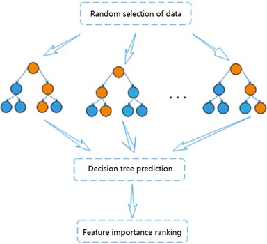
Random forest is a highly flexible integrated machine learning algorithm [11], which consists of a combination of multiple decision trees. Each decision tree can be considered as a classifier and is not correlated with each other. For each sample of the input, $N$ decision trees produce their respective $N$ results. and the results of each decision tree will be integrated to play a common role, reflecting the idea of Bagging [12]. The importance of each feature will be generated when the random forest model is established, and the features with strong importance will be selected [13]. Fig. 3 shows the flow chart of the random forest algorithm.

Through self-service sampling technology, the algorithm randomly selects $m$ samples from the training sample set in the original data to generate a new sample training set (The sample is put back in after each selection). The dimension of each sample is $a$ , and then $n$ features are randomly selected from the training set to form a decision tree. Repeat the above steps, and finally classification or prediction results is obtained. Based on the highly accurate prediction results obtained, the ranking of the degree of influence of each variable on the activity of the dependent compound can be further analyzed by observing the number of weights of each molecular descriptor. The ranking for feature importance can be further divided into ranking based on impurity and accuracy, and the degree of influence of the independent variables on the dependent variable is determined based on the influence of each variable change on the impurity and accuracy of the results.

Fig. 3Flow chart of random forest algorithm

The key in the algorithm is to determine the nodes of the decision tree according to the Gini coefficients [14], which can be defined as:

2

G i n i (t) = 1 - \sum_{j}^{N} [p (j | t)]^{2},

$p (j | t)$ is the probability of class label $j$ at node $t$ . When the Gini coefficient takes the minimum value of 0, all records at $t$ belong to the same class, indicating that the most useful information can be obtained. When node $t$ is split by $k$ sub-nodes, the split Gini coefficient is:

3

G i n i_{s p l i t} = \sum_{i = 1}^{k} \frac{N_{i}}{N} G i n i (i),

where $N_{i}$ is the number of records of the $i$ -th child node and $N$ is the number of records of the parent node $t$ . The random forest is constructed from the decision tree, and the features are selected according to the random forest.

The specific steps of the algorithm are as follows.

1) Randomly select $m$ sample subsets from the training set as the root node samples of each tree;

2) Build a decision tree based on these $m$ sample subsets, randomly select $n$ features to be selected, and from which the best attributes are selected as split nodes to complete the split;

3) Repeat the above two steps until a preset threshold is reached and each decision tree is fully grown;

4) Repeat the above three steps until the preset number of trees is reached, i.e. regress each decision tree of the test sample, and finally take the arithmetic mean of all results as the final output result of the model;

5) Based on the importance coefficients of each feature in the prediction results, the feature ranking of the molecular descriptors is then obtained.

In the random forest Boosting algorithm, feature importance is to reorder the original $m$ samples and $n$ feature values continuously, and check their impact on the regression results to further identify the features that have a significant impact on the target.

3.3. Random forest model solving

After preprocessing the data set with numerical type detection and normalization, the random forest algorithm is selected to analyze the importance of the effect of each independent variable on the activity of the compounds. The training set and test set are divided according to the ratio of 7:3. Based on the sklearn.RandomForestRegressor library provided by Python language, a random forest algorithm model is established for regression analysis to get the weight vector of data indicators $W = (w_{1}, w_{2}, . . ., w_{n})$ , $w_{i} \in R^{+}$ , and then the final feature ranking vector is obtained $R = (r_{1}, r_{2}, \dots, r_{m})$ , whose absolute value is the degree of influence of each variable on the pIC₅₀ value, and the top twenty molecular structure descriptors with the most significant influence on the pIC₅₀ value are shown in the Table 1.

Table 1The top twenty molecular structure descriptors with the most significant influence on the pIC50

No.	Molecular structure descriptors	Level of importance	No.	Molecular structure descriptors	Level of importance
1	minsssN	0.2533	11	VC-5	0.0209
2	LipoaffinityIndex	0.1706	12	nHBAcc	0.0088
3	MDEC-23	0.1187	13	minHBint5	0.0047
4	maxHsOH	0.1055	14	minsOH	0.0039
5	minHsOH	0.0911	15	hmin	0.0024
6	MLFER_A	0.0766	16	ATSc2	0.0020
7	C1SP2	0.0353	17	BCUTp-1h	0.0017
8	maxssO	0.0324	18	ATSc3	0.0011
9	MLogP	0.0312	19	MDEC-33	0.0009
10	BCUTc-1l	0.0264	20	TopoPSA	0.0009

Bar chart of the feature importance scores corresponding to the top 20 molecular structure descriptors with the most significant impact on biological activity is as follows Fig. 4.

Fig. 4Top 20 molecular descriptors in terms of importance

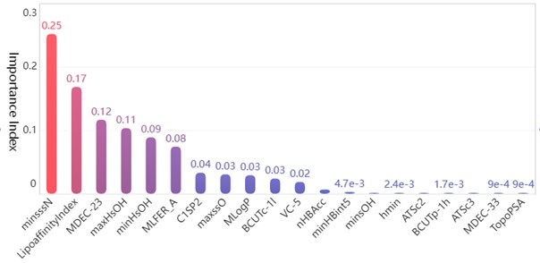
Among the obtained results, the molecular body minsssN has the highest weight on the pIC₅₀ value with 25.33 %. Next, the influence of LipofaffinitityIndex on the pIC₅₀ value has also reached 17.06 %. The top 20 molecular structures with the greatest influence on the pIC₅₀ value add up to 98.84 % of the importance, while the other 709 molecular structures account for only 1.16 %. There are 11 molecular structures with importance above 2 %, accounting for a total of 94.11 %. It is enough to show that these 20 molecular structures have an influence on the pIC₅₀ value.

The mean squared error (MSE) is used as the regression index after applying the model to obtain predicted values in the test set and comparing them with the true values [15]:

4

M S E = \frac{1}{N} {\sum_{i = 1}^{N} ({o b s e r v e d}_{i} - {p r e d i c t e d}_{i})}^{2} .

In the above formula observed is the true value and predicted is the predicted value. The MSE of the model line running on the test set is 0.03684, which indicates that the model achieves a good regression effect. According to the algorithmic characteristics of the random forest regression algorithm, it can be seen that each feature is obtained by weighted summation. The larger the absolute value of the weighting coefficient is, the more important the corresponding feature is, so this screening method is reasonable. Finally, the 20 molecular structure descriptors that have a greater weight on the pIC₅₀ value screened by this method are also reasonable.

4. Random forest-based molecular structure descriptor screening

4.1. Overview of support vector regression algorithm

Support vector regression algorithm is an application of support vector machine algorithm in the face of regression problems [16]. The support vector machine algorithm is a machine learning algorithm based on the principle of structural risk minimization, and its basic idea is to find an optimal surface between two classes of samples, so that the error of each sample in the two classification sets is minimized, but the distance of the classification intervals between the two classification sets is maximized. However, in this instance, considering the large dimensionality of the sample data, three cases of sample points linearly divisible, approximately linearly divisible, and linearly indivisible are tested separately. If linearly indivisible, a kernel function is introduced to map the high-dimensional sample data to the low-dimensional, so as to find the optimal surface of classification in the sample data [17, 18].

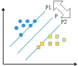
The linear separable case means that there exists an optimal classification surface P that can separate two types of sample points with different properties in the sample. P1 and P2 surfaces pass through some of the sample points and these two surfaces are parallel to the H surface, and the points on P1 and P2 surfaces are the nearest points to the rightmost surface, and the distance between P1 and P2 surfaces is defined as the classification interval, and the points falling on the two parallel lines are the support vectors. The specific representation is shown in the following Fig. 5.

Fig. 5Support vector machine schematic

If the sample is linearly differentiable, the sample set can be assumed to be $(x_{i}, y_{i})$ , $i = 1,2, . . ., n$ ; $x_{i} \in R^{d}$ , $y_{i} \in {+ 1, - 1}$ , where $+ 1$ and $- 1$ denote sample categories. $x_{i}$ will be classified. If $x_{i}$ is within the first class of sample points, $y_{i}$ is denoted as $+ 1$ , and if $x_{i}$ is within the second class of sample points, $y_{i}$ is denoted as $- 1$ . After normalizing the parameters, a corresponding inequality is obtained to constrain the set of samples to be classified, as shown in the following Eq. (5):

5

y_{i} [(ω \cdot x_{i}) + b] - 1 \geq 0, i = 1,2, \dots, n,

where $ω$ satisfies the equation $ω \cdot x + b = 0$ . From this, we can know that the interval between the two parallel lines P1 and P2 is $2 / ‖ω‖$ . If the sample satisfies the constraint of Eq. (4), the classification error rate is zero, so if the classification interval is larger, the empirical risk is smaller. Thus, the sample classification problem is quantified in such a way that the classification is better when the value of $‖ω‖$ is minimized.

After transforming the above problem into a problem of minimizing structural risk, the specific formula is as follows:

6

\min \frac{1}{2} {‖ω‖}^{2},

s . t . y_{i} ((ω \cdot x_{i}) + b) \geq 1, i = 1,2, . . ., n .

The Lagrangian approach transforms the above problem into a dual problem:

7

L = \frac{1}{2} {‖ω‖}^{2} - \sum_{i = 1}^{n} α_{i} [y_{i} (ω \cdot x_{i} + b) - 1],

where $a$ is $α_{1}$ non-negative Lagrange multiplier. Then the dual problem of the optimization problem is obtained as follows:

8

\max \sum_{i = 1}^{n} α_{i} - \frac{1}{2} \sum_{i = 1}^{n} \sum_{j = 1}^{n} α_{i} α_{j} y_{i} y_{j} (x_{i} \cdot x_{j}),

s . t . \sum_{i = 1}^{n} a_{i} y_{i} = 0, a_{i} \geq 0, i = 1,2, . . ., n .

In general $α_{i} = 0$ and then the sample corresponding to $α_{i} \neq 0$ is called support vector machine.

The approximately linearly divisible case means that when the above case is not divisible, a non-negative relaxation variable can be introduced to transform Eq. (7) into:

9

y_{i} [(ω \cdot x_{i}) + b] - 1 + ζ_{i} \geq 0, i = 1,2, . . ., n .

$ζ_{i}$ is an allowable deviation from the optimal classification surface. Thus, the original problem can be modified as follows:

10

\min \frac{1}{2} {‖ω‖}^{2} + c \sum_{i - 1}^{n} ζ_{i},

s . t . y_{i} ((ω \cdot x_{i}) + b) \geq 1 - ζ_{i} {, ζ}_{i} \geq 0, i = 1,2, . . ., n,

where $c$ is a penalty parameter, indicating the degree of punishment for classification errors in the classification process. The larger the $c$ value is, the higher the classification accuracy is, and the smaller the $c$ value, the lower the classification accuracy. However, the larger the value of $c$ is, the more difficult it is to classify the model, so a middle value should be found to achieve the best adaptability and accuracy of the model calculation.

The linear indivisible case refers to the fact that some problems may not find an optimal classification surface in real life, so it is necessary to use a nonlinear mapping $φ$ to process the sample set and map the samples to a higher dimension, so that they can be linearly divisible in this high-dimensional space. Therefore define $φ$ as:

11

φ : x {\subset y}_{i} R^{d} \to φ (x) \subset H .

Similar to the approximately linearly divisible problem, a classification surface is constructed in a high-dimensional space:

12

ω \cdot φ (x) + b = 0 .

$ω, b (ω \in H, b \in R)$ correspond to the solutions of the following optimization problems:

13

\min \frac{1}{2} {‖ω‖}^{2} + c \sum_{i - 1}^{n} ζ_{i},

s . t . y_{i} ((ω \cdot {φ (x)}_{i}) + b) \geq 1 - ζ_{i}, ζ_{i} \geq 0, i = 1,2, . . ., n .

The corresponding dual problem is:

14

\max \sum_{i - 1}^{n} α_{i} - \frac{1}{2} \sum_{i - 1}^{n} \sum_{j - 1}^{n} α_{i} α_{j} y_{i} y_{j} (x_{i} \cdot x_{j}),

s . t . \sum_{i - 1}^{n} a_{i} y_{i} = 0, 0 \leq a_{i} \leq c, i = 1,2, . . ., n .

$K (x_{i} \cdot x_{j}) = φ (x_{i}) φ (x_{j})$ is called the kernel function and $φ (x_{i})$ is the basis function. Then the final decision function is obtained as:

15

f (x) = sgn (\sum_{i = 1}^{n} α_{i} y_{i} K (x_{i}, x) + b) .

The problem of finding the optimal classification surface is solved by introducing the kernel functions.

There are various types of kernel functions [19], and the commonly used kernel functions include linear kernel functions, polynomial kernel functions, radial basis kernel functions, and Sigmoid kernel functions. Different choices of kernel functions will have an impact on the prediction results, and the specific formulas for each type of kernel function are shown below.

Linear kernel functions:

16

K (x, x_{i}) = x^{T} x_{i} .

Polynomial kernel functions:

17

K (x, x_{i}) = (g x^{T} x_{i} + r)^{d} .

Radial basis kernel functions:

18

K (x, x_{i}) = \exp (- \frac{{‖x - x_{i}‖}^{2}}{2 σ^{2}}) .

Sigmoid kernel function:

19

K (x, x_{i}) = \tanh (g x^{T} x_{i} + r) .

4.2. Kernel function solution for support vector regression models

Support vector machine regression is first performed on the 1974 data sets in the test set based on the 20 influencing factors selected in the previous. Then the Linear kernel function, radial basis kernel function, Sigmoid kernel function and polynomial kernel function are cross-validated to compare the advantages and disadvantages of the prediction results of support vector machines built by various kernel functions. In the process of building support vector regression models for each kernel function, a grid search method is used for parameter iteration to obtain the parameters that make the prediction results most accurate. The effect of support vector regression tuning for each type of kernel function is represented in the following Fig. 6.

Fig. 6Example of figure consisting of multiple charts

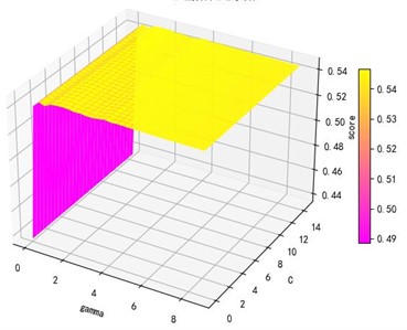
a) Kernel function parameters and R2 diagram

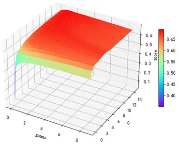
b) kernel function parameters and R2 diagram

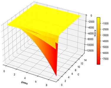
c) Sigmoid kernel function parameters and R2 diagram

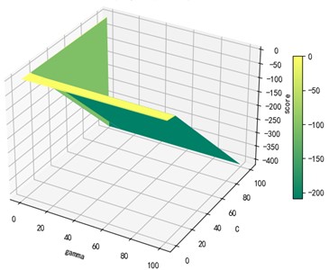
d) Polynomial kernel function parameters and R2 diagram

The trend of the support vector machine regression prediction results under each type of kernel function changing with the values of the parameters Gamma and can be seen from the four sets of images. By comparison, it is obvious that in the support vector machine model using polynomial kernel function $R ²$ rapidly decreases to below –200 with the change of parameter c value; when using Sigmoid kernel function with the change of parameter Gamma value $R ²$ rapidly decreases to below –700; when using Linear kernel function with the change of parameter Gamma value and c value $R ²$ is between 0.49 and 0.55. As $R ²$ is generally above 0.65 with the change of the parameter gamma and c values, The support vector machine model with radial basis kernel function has the best prediction fit. After the parameter tuning of the above four kernel functions, the parameter gamma and c values of each function in its optimal case and their corresponding prediction correlation coefficients are shown in the following Table 2.

Table 2Kernel function parameters and fitting degree

Kernel functions	Gamma	$c$	$R^{2}$
Linear	0.0100	3.0100	0.6467
Radial basis	8.9099	2.5100	0.9316
Sigmoid	0.0100	14.5100	0.6347
Polynomial	1.0000	0.0100	0.5379

The configuration of the equipment used in this experiment is: CPU is intel Core i5-6300HQ @ 2.30GHz; Memory is 12GB; GPU is NVIDIA GeForce RTX960M; Operating system is Windows 10 Professional Edition and Python version is 3.7.9. For different kernel functions, the grid search method [20] takes different time to find the optimal parameters, and the training time for each kernel function is shown in the following table.

Table 3Training schedules for different kernel functions or models

Kernel functions	Training time (hours)
Linear	2.17
radial basis	0.72
Sigmoid	1.29
Polynomial	1.77

After finding the best parameters of the support vector regression model under the four kernel functions, $R ²$ is used as the evaluation index of the prediction results, and its value ranges from [0,1]. the closer $R ²$ is to 1, the better the performance of the model is indicated. By comparison, it is found that the support vector regression model with radial basis function as kernel function has the best fit at a Gamma value of 8.9099 and a c value of 2.5100. The radial basis SVR model after determining the above tuning parameters is trained on the training set data, and the fitting results are obtained as shown below.

Fig. 7Example of figure consisting of multiple charts

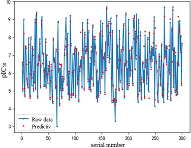
a) a) Training set fitting effect diagram

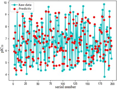
b) Test set fitting effect diagram

The support vector regression model based on the radial basis kernel function has good results in both the training and test sets. The fitting degree $R^{2}$ of the model in the training set is 0.9316, and the mean variance is 0.3732; the fitting degree $R^{2}$ of the model reached 0.7047 In the test set, and the mean variance is 0.6215. The fitting effect obtained by using RBF kernel function is far better than the other three kernel functions. At the same time, the training time of the support vector regression model using the radial basis function as the kernel function is also the fastest, with an average of only 0.72h. In addition, compared with references [8] and [9] mentioned in the introduction, the $R ²$ of the support vector regression model based on the Radial basis function kernel function is 0.23 higher than the multiple linear regression model mentioned in reference [8], and 0.17 higher than the Random forest model mentioned in reference [9]. It can be seen that the support vector regression model based on radial basis function kernel has good fitting accuracy and robustness, and has significant advantages in running time compared to other kernel functions. It can provide a reliable solution for further application to other drug screening.

5. Conclusions

In the experiment, a new idea is proposed, that is, the original mapping from the compound to the degree of biological activity is disassembled. The machine learning method is used to establish a new mapping relationship from the molecular structure of the compound to the degree of biological activity, screen out the molecular structure that has the greatest impact on biological activity, and then use the molecular structure as an intermediate bridge to reconnect the impact of the compound on biological activity.

In the process, a random forest regression model with high generalization ability and accuracy is selected to screen out the top 20 molecular structures from a total of 729 according to the importance of their effects on biological activity. The weight of the top 20 molecular structures’ influence on biological activity is 98.84 % in total, while the other 709 structures only account for 1.16 % in total. Basically, it can be concluded that only the top 20 molecular structures screened have an effect on biological activity. Then the support vector regression models under four kernel functions are compared in terms of effect and training time, and finally the support vector regression model with radial basis function as the kernel function is selected. Finally, the prediction model from compound to biological activity value is established. The model can realize the fitting of high-dimensional data by relying on a small number of data samples, and has better accuracy and shorter training time than using other functions as kernel functions.

Through the random forest and support vector regression model, the molecular structure descriptors of the compound is taken as the direct influencing factors, and the effect of small molecules on the target biological activity value can be used to predict the target biological activity value under the action of compounds. Since few anticancer drugs are currently used in the clinical phase and their effects are not particularly significant, a machine learning-based approach is proposed to screen compounds with high biological activity from a large number of compounds. It can not only provide theoretical support for future clinical experiments, but also reduce the scope of experiments in drug experiments and save a lot of time and cost, which is of great significance.

References

H. Sung et al., “Global Cancer Statistics 2020: GLOBOCAN estimates of incidence and mortality worldwide for 36 Cancers in 185 Countries,” CA: A Cancer Journal for Clinicians, Vol. 71, No. 3, pp. 209–249, May 2021, https://doi.org/10.3322/caac.21660

Publisher
A. Mohanty, R. R. Pharaon, A. Nam, S. Salgia, P. Kulkarni, and E. Massarelli, “FAK-targeted and combination therapies for the treatment of cancer: an overview of phase I and II clinical trials,” Expert Opinion on Investigational Drugs, Vol. 29, No. 4, pp. 399–409, Apr. 2020, https://doi.org/10.1080/13543784.2020.1740680

Publisher
A. Kalyanaraman et al., “Tamoxifen induces stem-like phenotypes and multidrug resistance by altering epigenetic regulators in ERα+ breast cancer cells,” Stem Cell Investigation, Vol. 7, pp. 20–20, Nov. 2020, https://doi.org/10.21037/sci-2020-020

Publisher
M. de Oliveira Vinícius et al., “pH and the breast cancer recurrent mutation D538G affect the process of activation of estrogen receptor α,” in Biochemistry, 2022, https://doi.org/10.1021/acs.biochem

Publisher
Lei Tian et al., “Exposure to PM2.5 enhances the PI3K/AKT signaling and malignancy of ERα expression-dependent non-small cell lung carcinoma,” Biomedical and Environmental Sciences: BES, Vol. 34, No. 4, pp. 319–323, Apr. 2021, https://doi.org/10.3967/bes2021.041

Publisher
W. Bingjie, S. Yinghui, L. Tianyu, and L. Tan, “ERα promotes transcription of tumor suppressor gene ApoA-l by breast cancer cells,” Journal of Zhejiang University-Science B (Biomedicine and Biotechnology), Vol. 22, No. 12, pp. 1034–1045, 2021.

Publisher
W. Qiang, “Tamoxifen activates ER α 36 Enhancement of breast cancer metastasis and its mechanism,” (in Chinese), Third Military Medical University, 2015.

Search CrossRef
D. Xueping, “ER based on machine learning method α prediction of inhibitor activity,” (in Chinese), Science and Technology Innovation, No. 11, pp. 1–4, 2022.

Search CrossRef
H. Yi, M. Shuangbao, and S. Biao, “ER based on random forest α bioactivity prediction research,” (in Chinese), Journal of Wuhan Textile University, Vol. 35, No. 4, pp. 54–56, 2022.

Search CrossRef
A. A. Hancock, E. N. Bush, D. Stanisic, J. J. Kyncl, and C. T. Lin, “Data normalization before statistical analysis: keeping the horse before the cart,” Trends in Pharmacological Sciences, Vol. 9, No. 1, pp. 29–32, Jan. 1988, https://doi.org/10.1016/0165-6147(88)90239-8

Publisher
D. S. Luz, T. J. B. Lima, R. R. V. Silva, D. M. V. Magalhães, and F. H. D. Araujo, “Automatic detection metastasis in breast histopathological images based on ensemble learning and color adjustment,” Biomedical Signal Processing and Control, Vol. 75, p. 103564, May 2022, https://doi.org/10.1016/j.bspc.2022.103564

Publisher
C. Wang, J. Du, and X. Fan, “High-dimensional correlation matrix estimation for general continuous data with Bagging technique,” Machine Learning, Vol. 111, No. 8, pp. 2905–2927, Aug. 2022, https://doi.org/10.1007/s10994-022-06138-3

Publisher
W. Guo, J. Zhang, D. Cao, and H. Yao, “Cost-effective assessment of in-service asphalt pavement condition based on Random Forests and regression analysis,” (in Chinese), Construction and Building Materials, Vol. 330, No. 11, p. 127219, May 2022, https://doi.org/10.1016/j.conbuildmat.2022.127219

Publisher
T. S. Biró, A. Telcs, M. Józsa, and Z. Néda, “f-Gintropy: an entropic distance ranking based on the Gini index,” Entropy, Vol. 24, No. 3, p. 407, Mar. 2022, https://doi.org/10.3390/e24030407

Publisher
Z. Qing, J. Ni, Z. Li, and J. Chen, “An improved mean-square performance analysis of the diffusion least stochastic entropy algorithm,” (in Chinese), Signal Processing, Vol. 196, p. 108512, Jul. 2022, https://doi.org/10.1016/j.sigpro.2022.108512

Publisher
H. Huang, X. Wei, and Y. Zhou, “An overview on twin support vector regression,” (in Chinese), Neurocomputing, Vol. 490, pp. 80–92, Jun. 2022, https://doi.org/10.1016/j.neucom.2021.10.125

Publisher
V. Vapnik, E. Levin, and Y. L. Cun, “Measuring the VC-dimension of a learning machine,” Neural Computation, Vol. 6, No. 5, pp. 851–876, Sep. 1994, https://doi.org/10.1162/neco.1994.6.5.851

Publisher
A. Daemen et al., “Improved modeling of clinical data with kernel methods,” Artificial Intelligence in Medicine, Vol. 54, No. 2, pp. 103–114, Feb. 2012, https://doi.org/10.1016/j.artmed.2011.11.001

Publisher
S. Abdollahi, H. R. Pourghasemi, G. A. Ghanbarian, and R. Safaeian, “Prioritization of effective factors in the occurrence of land subsidence and its susceptibility mapping using an SVM model and their different kernel functions,” Bulletin of Engineering Geology and the Environment, Vol. 78, No. 6, pp. 4017–4034, Sep. 2019, https://doi.org/10.1007/s10064-018-1403-6

Publisher
X. Jiang and C. Xu, “Deep learning and machine learning with grid search to predict later occurrence of breast cancer metastasis using clinical Data,” Journal of Clinical Medicine, Vol. 11, No. 19, p. 5772, Sep. 2022, https://doi.org/10.3390/jcm11195772

Publisher

About this article

Received

27 March 2023

Accepted

19 September 2023

Published

04 November 2023

DOI

https://doi.org/10.21595/chs.2023.23292

Keywords

drug screening

random forest regression

radial basis kernel function

support vector machine

Acknowledgements

The authors have not disclosed any funding.

Data Availability

The datasets generated during and/or analyzed during the current study are available from the corresponding author on reasonable request.

Author Contributions

Ke Jin is the author of the methods involved in this article, the author of the experiment, and the author of the paper. Cunqing Rong summarized and reviewed the literature, and pointed out the prospects and deficiencies. Jincai Chang put forward the question of the research and approved the final manuscript.

Conflict of interest

The authors declare that they have no conflict of interest.

This is an open access article distributed under the Creative Commons Attribution License, which permits unrestricted use, distribution, and reproduction in any medium, provided the original work is properly cited.

Previous article in issue Previous Next article in issue Next

Research article

2023 05 05

Predicting flow in porous media: a comparison of physics-driven neural network approaches

Shankar Lal Dangi, Viltė Karaliūtė, Neetish Kumar Maurya, Mayur Pal

Research article

2020 11 21

Performance evaluation method of spherical bearing based on correlation and sensitivity analysis and SVM

Chen Liu, Yongjun Ni, Erli Gao, Wenxue Song

Research article

2019 04 25

Remaining useful life (RUL) prediction of bearing by using regression model and principal component analysis (PCA) technique

Apakrita Tayade, Sangram Patil, Vikas Phalle, Faruk Kazi, Satvasheel Powar

Research article

2019 02 15

Performance optimization of banana vibrating screens based on PSO-SVR under DEM simulations

Zhanfu Li, Kunyuan Li, Xiaole Ge, Xin Tong

K. Jin, C. Rong, and J. Chang, “Application of machine learning algorithms in drug screening,” Journal of Complexity in Health Sciences, Vol. 6, No. 2, pp. 35–48, Nov. 2023, https://doi.org/10.21595/chs.2023.23292

Copy Extrica

Copied to clipboard!

TY  - JOUR
DO  - 10.21595/chs.2023.23292
UR  - https://doi.org/10.21595/chs.2023.23292
TI  - Application of machine learning algorithms in drug screening
T2  - Journal of Complexity in Health Sciences
AU  - Jin, Ke
AU  - Rong, Cunqing
AU  - Chang, Jincai
PY  - 2023
DA  - 2023/11/04
PB  - JVE International Ltd.
SP  - 35-48
VL  - 6
IS  - 2
SN  - 2538-7995
SN  - 2538-8002
ER  - 

Copy Ris

Copied to clipboard!

 @article{Jin_2023, title={Application of machine learning algorithms in drug screening}, volume={6}, ISSN={2538-8002}, url={https://doi.org/10.21595/chs.2023.23292}, DOI={10.21595/chs.2023.23292}, number={2}, journal={Journal of Complexity in Health Sciences}, publisher={JVE International Ltd.}, author={Jin, Ke and Rong, Cunqing and Chang, Jincai}, year={2023}, month=nov, pages={35–48} }

Copy Bibtex

Copied to clipboard!

[1]K. Jin, C. Rong, and J. Chang, “Application of machine learning algorithms in drug screening,” Journal of Complexity in Health Sciences, vol. 6, no. 2, pp. 35–48, Nov. 2023, doi: 10.21595/chs.2023.23292.

Copy IEEE

Copied to clipboard!

Jin, Ke, Cunqing Rong, and Jincai Chang. “Application of Machine Learning Algorithms in Drug Screening.” Journal of Complexity in Health Sciences 6, no. 2 (November 4, 2023): 35–48. https://doi.org/10.21595/chs.2023.23292.

Copy Chicago

Copied to clipboard!

Application of machine learning algorithms in drug screening

Abstract

Highlights

1. Introduction

2. Data overview and preprocessing

2.1. Data overview

2.2. Data pre-processing

3. Random forest-based molecular structure descriptor screening

3.1. Experimental process

3.2. Overview of random forest algorithm

3.3. Random forest model solving

4. Random forest-based molecular structure descriptor screening

4.1. Overview of support vector regression algorithm

4.2. Kernel function solution for support vector regression models

5. Conclusions

References

About this article

Related Articles