Abstract
Obesity, characterized by excess adipose tissue, is becoming a major public health problem. This condition, caused primarily by unbalanced energy intake (overconsumption) and exacerbated by modern lifestyles such as physical inactivity and suboptimal dietary habits, is the harbinger of a variety of health disorders such as diabetes, cardiovascular disease, and certain cancers. Therefore, there is an urgent need to accurately diagnose and assess the extent of obesity in order to formulate and apply appropriate preventive measures and therapeutic interventions. However, the heterogeneous results of existing diagnostic techniques have triggered a fierce debate on the optimal approach to identifying and assessing obesity, thus complicating the search for a standard diagnostic and treatment method. This research primarily aims to use machine learning techniques to build a robust predictive model for identifying overweight or obese individuals. The proposed model, derived from a person's physical characteristics and dietary habits, was evaluated using a number of machine learning algorithms, including Multilayer Perceptron (MLP), Support Vector Machine (SVM), Fuzzy K-Nearest Neighbors (FuzzyNN), Fuzzy Unordered Rule Induction Algorithm (FURIA), Rough Sets (RS), Random Tree (RT), Random Forest (RF), Naive Bayes (NB), Logistic Regression (LR), and Decision Table (DT). Subsequently, the developed models were evaluated using a number of evaluation measures such as correlation coefficient, accuracy, kappa statistic, mean absolute error, and mean square error. The hyperparameters of the model were properly calibrated to improve accuracy. The study revealed that the random forest model (RF) had the highest accuracy of 95.78 %, closely followed by the logistic regression model (LR) with 95.22 %. Other algorithms also produced satisfactory accuracy results but could not compete with the RF and LR models. This study suggests that the pragmatic application of the model could help physicians identify overweight or obese individuals and thus accelerate the early detection, prevention, and treatment of obesity-related diseases.
1. Introduction
The World Health Organization (WHO) defines overweight and obesity as conditions characterized by abnormal or excessive fat accumulation in the human body with the potential to negatively affect a person's overall health. A common measure used to assess these conditions is the Body Mass Index (BMI), a calculated value derived by dividing a person’s weight (in kilograms) by the square of their height (in meters). A BMI of 25 or more is considered an indication of obesity, while a BMI of over 30 is considered obese. Obesity is a major public health problem and is associated with increased susceptibility to a number of health complications, including diabetes, cardiovascular disease, and certain cancers [1].
Obesity is a complex condition due to a number of factors, the most important of which is a mismatch between energy intake and energy expenditure. This mismatch affects numerous metabolic pathways, culminating in overactive adipogenesis and the subsequent accumulation of excess energy in the form of triglycerides. At the same time, other factors such as suboptimal nutrition, insulin resistance, systemic inflammation, and genetic predispositions play an important role in the development of obesity [2]-[7].
Genetic predisposition to obesity is a complex trait that affects both the human genome and the metagenomes of the microbiota that inhabit the human body. Certain genetic variations have been found to affect energy metabolism and appetite regulation, causing an imbalance between energy intake and consumption that eventually leads to obesity. In addition, there is growing evidence of the crucial role of the gut microbiome in the development of obesity, as certain bacterial strains have been linked to alterations in metabolism, inflammation, and appetite regulation, possibly contributing to the development of obesity [2], [8].
Despite the role played by genetic susceptibility to obesity, there is consensus in the scientific community that environmental factors are the main cause of today's obesity epidemic. Influences such as dietary habits, physical activity levels, and a sedentary lifestyle are important factors contributing to obesity. In addition, the gut microbiome, which responds to changes in diet and environment, has been shown to play a critical role in the development of obesity, particularly in adults. Although the composition of the gut microbiota is regulated at the genetic level, it can be significantly modulated by environmental variables such as diet. Numerous studies have found that diets high in fat, carbohydrates, and energy are major contributors to the global prevalence of obesity [9]-[11].
Currently, clinical strategies for the management of obesity focus primarily on alleviating the complications and comorbidities associated with this condition. These strategies usually involve a holistic approach of dietary modification, behavior change, and increased physical activity to facilitate weight loss and improve overall health. A common approach is to restrict calorie intake, often in conjunction with increased physical activity, to achieve a negative energy balance. Lifestyle changes, which include stress management, adequate sleep, and increased physical activity, are often recommended as part of a comprehensive treatment plan. In more severe cases where conventional measures prove ineffective, pharmaceutical options and bariatric surgery may be considered a last resort. The main goal of clinical interventions is to improve overall health and reduce the risks associated with obesity-related complications [12, 13].
Obesity is a major public health challenge as it is associated with a number of diseases such as diabetes, cardiovascular disease, and certain cancers. Body Mass Index (BMI), a calculation of a person's weight in kilograms divided by the square of their height in meters, is the predominant tool used to diagnose obesity. People with a BMI of more than 30 kg/m2 are classified as obese, while people with a BMI of more than 25 kg/m2 are considered overweight. Although BMI is widely used because of its simplicity and cost-effectiveness, it also has its limitations, particularly because it is unable to account for differences in muscle mass, bone density, and fat distribution. Therefore, additional methods such as skinfold thickness measurement, bioelectrical impedance, and dual-energy X-ray absorptiometry (DXA) are used to assess body fat and muscle mass [15].
BMI is routinely used as a preliminary and practical tool to detect obesity. According to the World Health Organization guidelines (WHO), a BMI above 25 is considered overweight, and a value above 30 is considered obese. However, recent studies show that the risk of chronic diseases in the population increases with a BMI value of 21. It is also known that the gut microbiota has a significant impact on metabolic health. Obesity is associated with numerous metabolic disorders, including type 2 diabetes, non-alcoholic fatty liver disease, cardiovascular disease, and malnutrition. Therefore, when assessing obesity and its associated health risks, it is critical to consider factors such as gut microbiota, body composition, and metabolic markers in addition to BMI [15]-[18].
Individuals who are classified as overweight or obese are at increased risk for numerous chronic diseases, including type 2 diabetes, cardiovascular disease, certain cancers, and sleep apnea. In addition, obesity can exacerbate conditions such as joint pain, osteoarthritis, and psychological problems such as depression and low self-esteem. Therefore, treating obesity is important not only for aesthetic reasons but also for overall health and well-being [16], [19].
Obesity is associated with an extensive range of chronic health ailments. Among these are:
– Type 2 diabetes: The risk of type 2 diabetes is heightened by obesity due to an increase in insulin resistance and a decrease in insulin sensitivity.
– Hypertension: Obesity serves as a prominent risk factor for hypertension, as excess weight burdens the heart and blood vessels, leading to elevated blood pressure.
– Cardiovascular disease: The probability of experiencing heart disease, stroke, and other cardiovascular conditions is amplified with obesity.
– Osteoarthritis: The extra strain placed on joints, particularly hips and knees due to obesity, often precipitates osteoarthritis.
– Depression: The probability of depression is amplified in the context of obesity, likely attributed to the physical and emotional repercussions of being overweight.
– Alzheimer's disease: An increased risk of developing Alzheimer's disease and other types of dementia is associated with obesity.
– Cancer: Obesity elevates the risk for several forms of cancer, including but not limited to breast, prostate, kidney, ovarian, liver, and colon cancer. It is essential to underscore that the health risks mentioned are merely representative of the numerous potential complications associated with obesity. As a result, the treatment and management of obesity are of paramount importance to mitigate the risk of these and other chronic health conditions [1], [7].
Efforts to prevent obesity require a holistic approach that encourages a healthy lifestyle, characterized by habitual physical activity and a balanced diet. Public policies, health education, and initiatives to promote health play an instrumental role in tackling the obesity problem. The precise determination of an individual's obesity severity is crucial for accurate diagnosis and personalized treatment. Machine learning emerges as a potent tool in this context, possessing the capability to predict individuals who could profit from specific diets or interventions. Machine learning algorithms are designed to distil information from data, and numerous research articles have attested to their efficacy in predicting and managing obesity [20]-[22].
Machine learning houses a repertoire of advanced algorithms proficient in analyzing and extracting information from extensive datasets. These algorithms can classify, fit, learn, predict, and analyze data, thereby enriching our understanding of obesity and our predictive capabilities. Machine learning algorithms are capable of identifying patterns and trends in data that may be complex or impossible for humans to discern, paving the way for early diagnosis, treatment, and management of obesity. Machine learning can also be leveraged to predict future outcomes, such as the likelihood of developing obesity-related health issues, aiding healthcare professionals in devising more effective interventions. Overall, machine learning has the potential to significantly enhance our understanding of obesity and contribute to the advancement of more efficacious prevention and treatment strategies [20], [23]-[25].
The healthcare sector has seen an upsurge of interest in the application of machine learning in recent years [27]. The aim of this study is to construct a predictive model employing machine learning techniques to swiftly identify and assess overweight or obese individuals. This model will be developed based on data pertaining to physical conditions and dietary habits, predicting an individual's likelihood of being obese and the severity of their obesity. This tool could prove advantageous for healthcare professionals in the early detection and intervention of obesity. The integration of machine learning in healthcare could enhance diagnostic and treatment outcomes, providing a more efficient approach for analyzing and interpreting voluminous data [28], [29].
This study is structured into various sections to present a lucid account of the research process and findings. Chapter 2 provides an overview of the experimental procedures, methodologies, and strategies utilized throughout the study, including data collection and pre-processing, the implemented machine learning algorithms, and the evaluation metrics employed. Chapter 3 elucidates the results achieved using the proposed machine learning classifiers, along with their performance and accuracy. Chapter 4 summarizes the research, emphasizing the main conclusions and recommendations for future work.
2. Materials and methods
The main goal of this study is to use machine learning methods to determine a person's level of obesity based on their dietary habits and physical condition in order to create personalized treatment plans for patients. In this research project, body mass index (BMI) is used as a determinant of obesity, which is then classified into different categories such as underweight, normal weight, overweight level I, overweight level II, obese type I, obese type II, and obese type III. This classification is based on equation (1) and follows the criteria of the World Health Organization (WHO) and the Mexican normative guidelines. Table 1 shows a comprehensive classification of BMI according to the WHO and the Mexican normative guidelines. The aim of this study is to develop a predictive model capable of accurately classifying individuals into these specified obesity categories, which could potentially aid in the early detection and intervention of obesity [28]:
Table 1BMI classification according to WHO and Mexican normativity [29]
Underweight | Less than 18.5 |
Normal | 18.5 to 24.9 |
Overweight | 25.0 to 29.9 |
Obesity I | 30.0 to 34.9 |
Obesity II | 35.0 to 39.9 |
Obesity III | Higher than 40 |
This study follows a structured methodology that can be explained in the following order:
1) Data collection: this involves compiling relevant information on the physical characteristics and dietary preferences of participants within a given population.
2) Data refinement: This phase involves the careful refinement of the collected data to eliminate missing or incongruent values, the calculation of the body mass index (BMI) for each person, and the classification of participants into different obesity strata according to World Health Organization (WHO) criteria and Mexican normative guidelines.
3) Implementation of machine learning models: In this phase, a set of machine learning algorithms such as Multilayer Perceptron (MLP), Support Vector Machine (SVM), Fuzzy K-nearest Neighbours (FuzzyNN), Fuzzy Unordered Rule Induction Algorithm (FURIA), Rough Sets (RS), Random Tree (RT), Random Forest (RF), Naive Bayes (NB), Logistic Regression (LR), and Decision Table (DT) are applied to the refined data.
4) Performance evaluation of the models: the resulting models are then examined using a number of performance indices such as Correlation Coefficient, Accuracy (ACC), Kappa Statistic (KS), Mean Absolute Error (MAE), Root Mean Square Error (RMSE) and Complexity Matrix.
5) Results and findings: This section explains the main findings of the study, especially with regard to the effectiveness of the different machine learning algorithms used.
6) Concluding remarks: This concluding section summarizes the main conclusions of the study and suggests possible future research in this area.
2.1. Dataset
The dataset used in this study [28] contains information that allows the degree of obesity of an individual to be assessed based on their dietary habits and physical condition. The dataset includes 2111 instances (rows) and 17 variables (columns) consisting of numeric, binary, and categorical input variables. A single target or outcome variable provides data on a person’s level of obesity. This data set, referred to as “NObesity”, includes the following classifications: Underweight, Normal Weight, Obesity Level I, Obesity Level II, Obesity Type I, Obesity Type II, and Obesity Type III. Table 2 provides a comprehensive overview of the data variables and includes variable names, data types, and precise definitions. The dataset is used to train and evaluate the machine learning models developed in this study to predict the level of obesity in individuals.
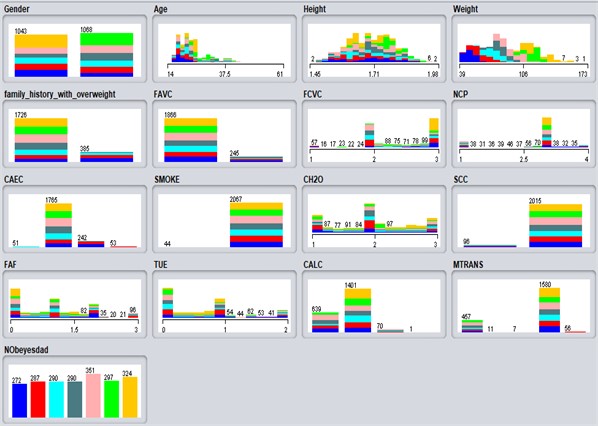
Each model input integrates a unique set of patient information along with a specific target variable. Input variables used in the model include demographic information, anthropometric measurements, and data on dietary habits and physical exertion. Fig. 1 shows the data distribution used to estimate a person's level of obesity based on their dietary habits and physical condition. This visualization illustrates the different contributions of each input variable to the prediction of the target variable, namely the level of obesity. It facilitates understanding of the relationship between the input variables and the target variable, as well as the relative importance of each variable in the prediction process. In addition, the figure shows the distribution of the data for each input variable, which can prove helpful in identifying the distribution of the data and any anomalies or patterns.
Table 2Dataset description
Attributes | Values |
Gender | 1 = Female or 0 = Male |
Age | Numeric |
Height | Numeric |
Weight | Numeric |
Family with overweight / obesity | 1 = Yes/ 0 = No |
FAVC (frequent consumption of high caloric food) | 0 = Yes/ 1 = No |
FCVC (frequent consumption of vegetables) | 1,2 or 3 |
NCP (number of main meals) | 1, 2, 3 or 4 |
CAEC (consumption of food between meals) | (1 = No, 2 = Sometimes, 3 = Frequently or 4 = Always) |
Smoke | 0 = Yes/ 1 = No |
CH20 (Consumption of water daily) | 1, 2 or 3 |
SCC (Calories consumption monitoring) | 0 = Yes/ 1 = No |
FAF (Physical activity frequency) | 0, 1, 2 or 3 |
TUE (Time using technology devices) | 0, 1 or 2 |
CALC (Consumption of alcohol) | 1 = No, 2 = Sometimes, 3 = Frequently or 4 = Always |
MTRANS (Transportation used) | Automobile, motorbike, bike, public transportation or walking |
Obesity level | 1 = Insufficient_Weight, 2 = Normal_Weight, 3 = Overweight_Level_I, 4 = Overweight_Level_II, 5 = Obesity_Type_I, 6 = Obesity_Type_II, 7 = Obesity_Type_III |
2.2. Machine learning algorithms
Machine learning (ML) is a rapidly advancing discipline that has attracted much attention in recent years. It involves the systematic study of algorithms and statistical models used by computer systems to perform tasks without the need for explicit programming. The ultimate goal of machine learning is to equip computers with the ability to use data more resourcefully and efficiently through a process known as reinforcement learning. This method allows computers to learn from data and incrementally improve their performance. Tools have always been used to perform a range of tasks more efficiently. With the increase in available data, the need for machine learning is becoming more acute. Machine learning is used to gain insights from vast amounts of data when traditional methods prove insufficient to decipher the information contained in the data. The development of autonomous learning robots that do not need to be explicitly programmed is a focus of current research. This could allow robots to adapt to variable environments and perform tasks more efficiently and effectively. Machine learning is used in a variety of sectors, including healthcare, finance, transportation, and manufacturing. It has the potential to revolutionize the way we live and work and offers ample opportunities for innovation and growth [21].
Fig. 1Graphical distributions of attributes by obesity level
The concept of “supervised learning classification” refers to the process of machine learning, where computer software is trained on a labeled data set, meaning that each input is assigned the correct output or class. The software then uses this training data to make predictions for new, unseen data. The goal of classification is to assign new observations to one of several predefined categories or classes. A variety of classification models can be used, such as decision trees, random forests, Naive Bayes, Support Vector machines, and logistic regression. Each model has its own strengths and weaknesses, and the choice of an appropriate model depends on the nature of the problem and the characteristics of the data. Classification techniques have applications in many fields, such as natural language processing, image recognition, and bioinformatics. They are also used in areas such as healthcare, finance, marketing, and customer relationship management. The purpose of classification is to divide large amounts of data into smaller groups based on common characteristics so that they are easier to understand and analyze. The classification model, which is similar to the regression model, predicts future outcomes and serves as an important method for examining data in various fields.
2.2.1. Multi-layer perceptron (MLP)
A multilayer perceptron (MLP) [30], [31], is a subset of feedforward artificial neural networks commonly used in supervised learning tasks such as classification and regression. The MLP consists of three main layers: an input layer, an output layer, and one or more hidden layers in between. The input layer primarily receives and processes input data, which is then passed through the network to the output layer. The output layer is responsible for producing the final prediction or output in response to the processed input data. The hidden layers, which lie between the input and output layers, contain neurons that perform computational tasks.
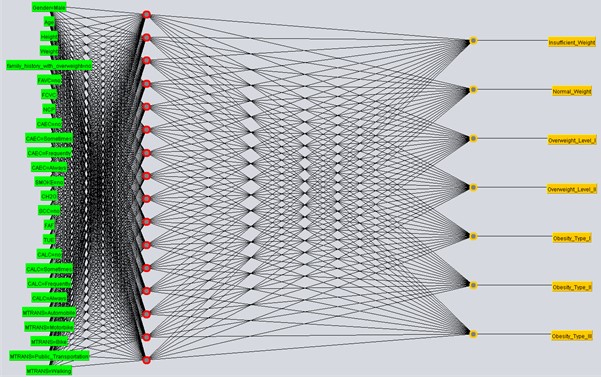
In the context of an MLP, the neurons are connected by weighted connections and use a non-linear activation function to process the incoming data. These connection weights are adjusted during the training phase to optimize the operational performance of the network. This process of changing the weights, called backpropagation, works like a supervised learning algorithm that applies gradient descent to minimize the error between predicted and actual output. MLPs are ideal for solving nonlinear problems because they can approximate any continuous function. They are used in a variety of fields, such as image recognition, natural language processing, and speech recognition [30-33]. The graphical user interface (GUI) of this classification algorithm, implemented with the software Weka, is shown in Fig. 2.
Fig. 2GUI of a multilayer perceptron for classification
2.2.2. Support vector machine (SVM)
Support Vector Machines (SVMs) [35] are a type of supervised learning algorithm commonly used for classification tasks. SVMs work by creating a boundary, called a “hyperplane”, that separates different classes of data points in a high-dimensional feature space. The primary goal of SVMs is to create a boundary that maximizes the distance from itself to the nearest data points in each class, providing an optimally separated hyperplane. SVMs are particularly effective in dealing with complicated and small to medium-sized data sets and are ideal for situations where the data is not linearly separable, i.e., cannot be divided by a single straight line.
For such scenarios, SVMs use a strategy called the kernel trick, which projects the data into a higher-dimensional space to facilitate linear separation. SVMs are used in a variety of machine learning domains, such as text classification, image classification, and bioinformatics. They have a solid theoretical foundation and have achieved exceptional experimental results. Since they are suitable for both classification and regression tasks, SVMs show high efficiency in processing linear and nonlinear data [34]-[36].
2.2.3. Fuzzy K-nearest neighbors (FuzzyNN)
The Fuzzy K-Nearest Neighbors (FKNN) algorithm is an adaptation of the traditional K-Nearest Neighbors (KNN) algorithm, an instance-based learning approach. FKNN uniquely integrates fuzzy logic with KNN to provide classification predictions. The main difference between FKNN and standard KNN is that FKNN uses a portion of the available samples in its architecture for predictions rather than the entire dataset.
This method of “instance-based learning” facilitates classification predictions by using a subset of samples within the FKNN structure. As a result, the algorithm requires less memory because it does not retain an array of abstractions distilled from specific instances. To alleviate this situation, the closest-neighbor algorithm has been improved.
The goal of this project is to prove that the memory requirements of FKNN can be significantly reduced while keeping the learning rate and classification accuracy as close as possible to their original values. This can be achieved by using a fraction of the accessible samples within the structure and applying fuzzy logic for predictions [37, 38].
2.2.4. Fuzzy unordered rule induction algorithm (FURIA)
The Fuzzy Unordered Rule Inductive Algorithm (FURIA) is an innovative algorithm for rule-based fuzzy classification that uses unordered rule sets for decision-making, unlike conventional rule lists. This relatively new advance in rule-based fuzzy classification offers several advantages over traditional methods [39].
One outstanding advantage of FURIA is its ability to generate concise and manageable rule sets, thus facilitating the interpretation and understanding of classification results. By using fuzzy rules and unordered rule sets instead of conventional rule lists, FURIA is able to take into account situations that might otherwise be overlooked. In addition, FURIA uses an optimal rule expansion mechanism that allows it to adapt to new circumstances and thereby improve classification accuracy.
Compared to other classifiers, such as the original RIPPER and C4.5, FURIA has shown a remarkable improvement in classification accuracy on test data. Consequently, FURIA proves to be an excellent tool for classification tasks with potential applications in various fields such as image recognition, natural language processing, and speech recognition [40], [41].
2.2.5. Rough sets (RS)
Rough sets (RS) are a mathematical framework for data processing and mining, a concept originally developed by Pawlak in the 1980s [42]. This pioneering approach extends traditional set theory by allowing the formulation of complex concepts that would otherwise be difficult to understand using standard reasoning paradigms. In rough set theory, a subset within a universal set is typified by ordered pairs of subsets and supersets belonging to the universal set itself.
An essential notion introduced by rough set theory is the concept of “approximate sets”, which derives from the equivalence between two different numerical sets. These approximate sets are further divided into upper and lower sets constructed using equivalence classes. These sets consist of the union of all equivalence classes that serve as subsets of a given set.
Rough sets have applications in various fields, including data mining, knowledge discovery, and decision-making. The ability to deal with the uncertainty and imprecision of data makes rough sets particularly advantageous in dealing with incomplete or inconsistent information. Furthermore, rough set theory underpins the theory of complete sets and has been instrumental in the development of novel algebraic structures [43, 44].
2.2.6. Random tree (RT)
Random Tree (RT) [46] is a methodological approach used in ensemble learning and is often used to tackle complex tasks in classification, regression, and similar domains. As a supervised classifier, it cultivates a large number of decision trees in the training phase, which are subsequently used to predict the class of new instances. Random trees are an example of a unique facet of ensemble learning, where numerous individual decision trees are cultivated and combined into a “random forest”, a collective of tree-based predictors.
This method proves particularly beneficial when processing high-dimensional and complex datasets, as it prevents overfitting and strengthens the generalization ability of the model. A key feature of random trees is that they combine the principles of single-model trees and random trees. In model trees, each leaf node is connected to a linear model that is optimized for the local subspace. In contrast, in random trees, the features and data samples are randomly selected during tree construction.
The ability to transform imbalanced trees into balanced trees through the use of random trees can greatly improve the precision and robustness of the model [47, 48].
2.2.7. Random forest (RF)
Random Forest is an ensemble learning technique that groups numerous decision trees together to solve different problems. In this paradigm, each tree is trained on a unique random subset of the data, and the matching decision or common value of these trees determines the output of the Random Forest. This method is particularly well suited for high-dimensional and complex datasets, as it prevents overfitting and improves the generalization performance of the model.
Training the individual trees on different random subsets of data helps to reduce the correlation between the trees and increase the diversity of the ensemble. This strategy, often referred to as “bagging” (or “bootstrap aggregation”) of decision trees, involves cultivating a comprehensive set of related trees to solve a given problem. In addition, the Random Forest algorithm includes a randomization element where each tree falls back on the values of an independently generated random vector. This feature increases the robustness of the model and provides protection against overfitting [46], [49], and [50].
2.2.8. Naive Bayes (NB)
Naive Bayes is a simplified learning method that goes back to Thomas Bayes [51]. It uses Bayes’ theorem and assumes robust conditional independence of features with respect to class. Although the independence assumption is not always satisfied in practical scenarios, Naive Bayes continues to be widely used due to its computational efficiency and other commendable properties.
The method works under the assumption that the characteristics used to estimate the value are independent of the value being estimated. Consider the case where the species of a fish is to be determined from its length and weight. In this context, the weight of a fish belonging to a particular species is usually dependent on its length and vice versa, possibly contradicting the assumption of independence. However, studies have shown that the independence assumption imposes fewer constraints on classification tasks involving categorical estimation than previously thought. In certain cases, unbiased Bayesian learning has led to lower error rates compared to more complicated learning strategies, such as the construction of univariate decision trees [52].
The quantitative component of a Bayesian network comprises three main elements: Probability theory, Bayes’ theorem, and conditional probability functions. Bayes' theorem is based on the idea that the conditional probability is proportional to the probability of an event occurring. This allows graphical models to conveniently represent probability distributions as conditional dependencies or independencies [53, 54].
2.2.9. Logistic regression (LR)
Logistic regression (LR) is a statistical method and supervised machine learning algorithm designed for analyzing and modeling the relationship between a binary or categorical dependent variable and one or more independent variables, typically manifested as continuous or categorical predictors. LR is often used for binary classification problems where the dependent variable has two potential outcomes or classes, such as success or failure, positive or negative, or the presence or absence of a particular condition.
The logistic regression model calculates the probability that the dependent variable can be assigned to a particular class depending on the values of the independent variables. The model uses the logistic function, also known as the sigmoid function, to convert linear combinations of predictors into probabilities that vary between 0 and 1. The model then applies these probabilities to make class predictions, using a threshold, usually 0.5, to determine the final class assignment.
The simplicity, interpretability, and ease of implementation of logistic regression contribute to its widespread use in various applications, such as medical diagnosis, customer loyalty prediction, and sentiment analysis. Moreover, logistic regression is less prone to overfitting compared to more complex machine learning models, especially when combined with regularization techniques such as L1 or L2 regularization. However, logistic regression requires a linear relationship between the logit of probabilities and the independent variables, a condition that is not always met in practice [55]-[58].
2.2.10. Decision table (DT)
Decision tables are a powerful tool for analyzing and understanding complex decision-making processes. They provide a structured and systematic representation of the relationships between different variables and the corresponding actions to be taken based on those variables. This makes decision tables particularly valuable in fields such as economics, finance, and computer programming, where effective decision-making plays a central role.
In addition, decision tables can be used to develop decision-making software and systems that automate the decision-making process according to the rules specified in the table. This streamlined approach increases the efficiency and consistency of decision-making across different applications and industries and enables more effective and reliable decision outcomes [59, 60].
3. Results
The results of the study show that the Random Forest (RF) classifier had the best performance in terms of accuracy, with a result of 95.78 %. The Logistic Regression (LR) classifier had the second-best performance with a result of 95.22 %. The Naive Bayes (NB) classifier achieved 67.41 %, while the Fuzzy NN classifier achieved 78.16 %. The Support Vector Machine (SVM) classifier achieved a result of 84.23 %, while the Decision Table (DT) classifier achieved a result of 84.89 %. The Random Tree (RT) classifier obtained a result of 87.3 %, while the Rough Set (RS) classifier obtained a result of 87.83 %. The multi-layer perceptron (MLP) classifier achieved 94.36 %, and the fuzzy unordered rule inductive algorithm (FURIA) achieved 95.07 %. Overall, the RF classifier was the most effective in accurately classifying and identifying obesity.
3.1. Performance evaluation
The main evaluation measures for classification problems include accuracy, precision, recognition, and the F1 score. Accuracy reflects the ratio of correctly classified instances to the total number of instances. Precision represents the proportion of correct positive predictions to all positive predictions. Recall, also referred to as sensitivity or “true-positive rate,” indicates the ratio of correct positive predictions to the total number of correct positive instances. The F1 score, a measure of a classifier’s balance between precision and recall, is calculated as the harmonic mean of precision and recall.
In addition to these metrics, ROC (Receiver Operating Characteristic) curves and AUC (Area under the Curve) are commonly used to evaluate the performance of binary classification models. ROC The curves illustrate the relationship between the rate of correct-positive predictions and the rate of false-positive predictions at different classification thresholds, while the AUC provides a comprehensive indicator of the classifier's performance by quantifying the area under the ROC curve.
The following table lists the criteria (equations) used in this study in order from Eqs. (1) to (9). For a detailed understanding of these formulae, please consult the relevant reference:
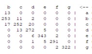
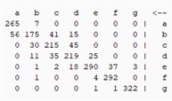
Several evaluation metrics derived from the confusion matrix are commonly used to evaluate the performance of classification models and facilitate comparisons between different models. A confusion matrix [71] or [72] is a tabular representation (see Table 3) that characterizes the performance of a classification algorithm. It is typically used in machine learning and statistics to evaluate the accuracy of a model in classifying a data set.
The confusion matrix is divided into four different categories: true-positive (TP), false-positive (FP), true-negative (TN), and false-negative (FN). True-positive (TP) refers to the number of correctly classified positive instances, while false-positive (FP) indicates the number of incorrectly classified positive instances. True-negative (TN) represents the number of negative instances that were correctly classified, and false-negative (FN) refers to the instances where negative classifications were inaccurately made.
Table 3Confusion matrix
Actual value | |||
Positive | Negative | ||
Predicted values | Positive | TP (True Positive) | FN (False Negative) |
Negative | FP (False Positive) | TN (True Negative) | |
Table 4Detailed accuracy by class
Alg. | TP Rate | FP Rate | Precision | Recall | F-Measure | MCC | ROC Area | PRC Area | Class |
MLP | 0.952 | 0.012 | 0.922 | 0.952 | 0.937 | 0.927 | 0.997 | 0.978 | Insufficient_Weight |
0.882 | 0.016 | 0.894 | 0.882 | 0.888 | 0.870 | 0.990 | 0.944 | Normal_Weight | |
0.869 | 0.013 | 0.913 | 0.869 | 0.890 | 0.874 | 0.985 | 0.929 | Overweight_Level_I | |
0.938 | 0.016 | 0.904 | 0.938 | 0.920 | 0.908 | 0.988 | 0.939 | Overweight_Level_II | |
0.977 | 0.006 | 0.972 | 0.977 | 0.974 | 0.969 | 0.998 | 0.990 | Obesity Tye I | |
0.980 | 0.002 | 0.986 | 0.980 | 0.983 | 0.980 | 0.997 | 0.990 | Obesity Tye II | |
0.994 | 0.000 | 1.000 | 0.994 | 0.996 | 0.996 | 0.998 | 0.996 | Obesity Tye III | |
SVM | 0.974 | 0.030 | 0.826 | 0.974 | 0.894 | 0.881 | 0.985 | 0.883 | Insufficient_Weight |
0.610 | 0.027 | 0.778 | 0.610 | 0.684 | 0.647 | 0.934 | 0.630 | Normal_Weight | |
0.741 | 0.043 | 0.734 | 0.741 | 0.738 | 0.696 | 0.938 | 0.650 | Overweight_Level_I | |
0.755 | 0.043 | 0.737 | 0.755 | 0.746 | 0.705 | 0.927 | 0.654 | Overweight_Level_II | |
0.826 | 0.017 | 0.906 | 0.826 | 0.864 | 0.840 | 0.957 | 0.811 | Obesity Tye I | |
0.983 | 0.021 | 0.885 | 0.983 | 0.931 | 0.921 | 0.986 | 0.877 | Obesity Tye II | |
0.994 | 0.002 | 0.991 | 0.994 | 0.992 | 0.991 | 0.997 | 0.988 | Obesity Tye III | |
FuzzyNN | 0.882 | 0.040 | 0.764 | 0.882 | 0.819 | 0.793 | 0.921 | 0.690 | Insufficient_Weight |
0.446 | 0.030 | 0.703 | 0.446 | 0.546 | 0.508 | 0.708 | 0.389 | Normal_Weight | |
0.676 | 0.038 | 0.740 | 0.676 | 0.706 | 0.663 | 0.819 | 0.544 | Overweight_Level_I | |
0.710 | 0.055 | 0.673 | 0.710 | 0.691 | 0.641 | 0.828 | 0.518 | Overweight_Level_II | |
0.786 | 0.050 | 0.758 | 0.786 | 0.772 | 0.726 | 0.868 | 0.632 | Obesity Tye I | |
0.949 | 0.035 | 0.817 | 0.949 | 0.879 | 0.860 | 0.957 | 0.783 | Obesity Tye II | |
0.994 | 0.007 | 0.961 | 0.994 | 0.977 | 0.973 | 0.993 | 0.956 | Obesity Tye III | |
FURIA | 0.967 | 0.004 | 0.970 | 0.967 | 0.969 | 0.964 | 0.995 | 0.980 | Insufficient_Weight |
0.895 | 0.018 | 0.889 | 0.895 | 0.892 | 0.875 | 0.966 | 0.886 | Normal_Weight | |
0.886 | 0.012 | 0.924 | 0.886 | 0.905 | 0.890 | 0.965 | 0.903 | Overweight_Level_I | |
0.959 | 0.014 | 0.914 | 0.959 | 0.936 | 0.926 | 0.991 | 0.955 | Overweight_Level_II | |
0.957 | 0.005 | 0.974 | 0.957 | 0.966 | 0.959 | 0.990 | 0.981 | Obesity Tye I | |
0.987 | 0.003 | 0.980 | 0.987 | 0.983 | 0.980 | 0.996 | 0.990 | Obesity Tye II | |
0.997 | 0.001 | 0.994 | 0.997 | 0.995 | 0.995 | 1.000 | 1.000 | Obesity Tye III | |
RS | 0.919 | 0.021 | 0.868 | 0.919 | 0.893 | 0.877 | 0.995 | 0.974 | Insufficient_Weight |
0.767 | 0.043 | 0.738 | 0.767 | 0.752 | 0.712 | 0.972 | 0.819 | Normal_Weight | |
0.769 | 0.015 | 0.892 | 0.769 | 0.826 | 0.803 | 0.979 | 0.922 | Overweight_Level_I | |
0.810 | 0.014 | 0.900 | 0.810 | 0.853 | 0.833 | 0.985 | 0.933 | Overweight_Level_II | |
0.889 | 0.015 | 0.923 | 0.889 | 0.906 | 0.887 | 0.992 | 0.968 | Obesity Tye I | |
0.980 | 0.009 | 0.948 | 0.980 | 0.964 | 0.958 | 0.999 | 0.995 | Obesity Tye II | |
0.997 | 0.026 | 0.875 | 0.997 | 0.932 | 0.922 | 1.000 | 0.999 | Obesity Tye III | |
RT | 0.904 | 0.014 | 0.904 | 0.904 | 0.904 | 0.890 | 0.945 | 0.833 | Insufficient_Weight |
0.742 | 0.038 | 0.755 | 0.742 | 0.749 | 0.710 | 0.855 | 0.599 | Normal_Weight | |
0.786 | 0.034 | 0.786 | 0.786 | 0.786 | 0.752 | 0.876 | 0.647 | Overweight_Level_I | |
0.834 | 0.032 | 0.807 | 0.834 | 0.820 | 0.791 | 0.901 | 0.696 | Overweight_Level_II | |
0.886 | 0.022 | 0.889 | 0.886 | 0.887 | 0.865 | 0.932 | 0.809 | Obesity Tye I | |
0.949 | 0.007 | 0.959 | 0.949 | 0.954 | 0.947 | 0.971 | 0.918 | Obesity Tye II | |
0.991 | 0.001 | 0.994 | 0.991 | 0.992 | 0.991 | 0.995 | 0.986 | Obesity Tye III | |
RF | 0.945 | 0.002 | 0.988 | 0.945 | 0.966 | 0.962 | 0.999 | 0.996 | Insufficient_Weight |
0.962 | 0.028 | 0.884 | 0.962 | 0.899 | 0.884 | 0.993 | 0.953 | Normal_Weight | |
0.897 | 0.005 | 0.963 | 0.897 | 0.929 | 0.918 | 0.994 | 0.974 | Overweight_Level_I | |
0.945 | 0.008 | 0.951 | 0.945 | 0.948 | 0.940 | 0.997 | 0.987 | Overweight_Level_II | |
0.966 | 0.004 | 0.980 | 0.966 | 0.973 | 0.967 | 0.999 | 0.997 | Obesity Tye I | |
0.987 | 0.002 | 0.990 | 0.987 | 0.988 | 0.986 | 1.000 | 0.999 | Obesity Tye II | |
0.997 | 0.001 | 0.997 | 0.997 | 0.997 | 0.996 | 1.000 | 1.000 | Obesity Tye III | |
NB | 0.897 | 0.047 | 0.737 | 0.897 | 0.809 | 0.783 | 0.979 | 0.860 | Insufficient_Weight |
0.484 | 0.056 | 0.577 | 0.484 | 0.527 | 0.462 | 0.914 | 0.582 | Normal_Weight | |
0.510 | 0.048 | 0.630 | 0.510 | 0.564 | 0.506 | 0.911 | 0.622 | Overweight_Level_I | |
0.483 | 0.082 | 0.484 | 0.483 | 0.484 | 0.402 | 0.878 | 0.473 | Overweight_Level_II | |
0.516 | 0.082 | 0.555 | 0.516 | 0.535 | 0.446 | 0.883 | 0.556 | Obesity Tye I | |
0.832 | 0.037 | 0.784 | 0.832 | 0.807 | 0.775 | 0.982 | 0.921 | Obesity Tye II | |
1.000 | 0.028 | 0.866 | 1.000 | 0.928 | 0.918 | 1.000 | 1.000 | Obesity Tye III | |
LR | 0.967 | 0.007 | 0.956 | 0.967 | 0.962 | 0.956 | 0.996 | 0.953 | Insufficient_Weight |
0.913 | 0.013 | 0.919 | 0.913 | 0.916 | 0.903 | 0.987 | 0.925 | Normal_Weight | |
0.907 | 0.013 | 0.916 | 0.907 | 0.912 | 0.898 | 0.983 | 0.858 | Overweight_Level_I | |
0.945 | 0.010 | 0.935 | 0.945 | 0.940 | 0.930 | 0.989 | 0.931 | Overweight_Level_II | |
0.963 | 0.005 | 0.974 | 0.963 | 0.968 | 0.962 | 0.990 | 0.970 | Obesity Tye I | |
0.973 | 0.005 | 0.970 | 0.973 | 0.971 | 0.967 | 0.987 | 0.961 | Obesity Tye II | |
0.991 | 0.003 | 0.985 | 0.991 | 0.988 | 0.985 | 0.997 | 0.987 | Obesity Tye III | |
DT | 0.897 | 0.028 | 0.824 | 0.897 | 0.859 | 0.838 | 0.994 | 0.960 | Insufficient_Weight |
0.791 | 0.021 | 0.853 | 0.791 | 0.821 | 0.795 | 0.973 | 0.856 | Normal_Weight | |
0.821 | 0.040 | 0.768 | 0.821 | 0.793 | 0.760 | 0.952 | 0.790 | Overweight_Level_I | |
0.755 | 0.034 | 0.779 | 0.755 | 0.767 | 0.731 | 0.962 | 0.788 | Overweight_Level_II | |
0.812 | 0.039 | 0.805 | 0.812 | 0.809 | 0.770 | 0.968 | 0.910 | Obesity Tye I | |
0.923 | 0.013 | 0.923 | 0.923 | 0.923 | 0.910 | 0.992 | 0.935 | Obesity Tye II | |
0.941 | 0.001 | 0.993 | 0.941 | 0.967 | 0.961 | 0.998 | 0.988 | Obesity Tye III |
The passage above describes a study in which machine learning algorithms were used to classify features associated with obesity and evaluate their performance. Several algorithms were used in the study, including MLP, SVM, FuzzyNN, FURIA, RS, RT, RF, NB, LR, and DT, which are well established in the field of categorization and have a solid performance history. The models were subjected to ten-fold cross-validation, and their results were presented in tables and graphs. The performance of the models was assessed in terms of accuracy, as shown in Table 4. Overall, the statement provides a comprehensive overview of the methodology and results of the study.
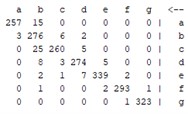
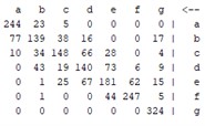
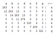
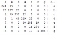
The above explanation provides a clear overview of how the confusion matrix is used to evaluate the performance of classification models and how it is used to calculate various performance measures. Table 5 shows that the results of the confusion matrix are given for all methods used, allowing a clear comparison of the performance of each method.
Table 5Confusion matrix for all models
MLP | SVM | FuzzyNN | FURIA |
 |  | 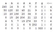 | 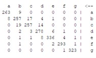 |
RS | RT | FR | NB |
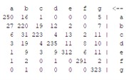 |  |  |  |
LR | DT | Definition | |
 |  |  | |
Other metrics such as the kappa statistic, the mean absolute error, and the root mean square error are also important indicators for the analysis of a classification task and were used in this study to compare the performance of the machine learning algorithms. The results of these evaluations are shown in the following figures.
Fig. 3Comparison of the accuracy of ten classifiers
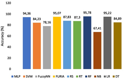
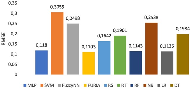
Analyzing these graphs, we can see that the performance of each ML algorithm varies in terms of accuracy (KS, MAE, and RMSE). The highest accuracy was achieved by the Random Forest (RF) algorithm with 95.78 %. The lowest accuracy was achieved by the Naive Bayes (NB) algorithm with 67.41 %. The graphs also show the comparison of the algorithms in terms of KS, MAE, and RMSE. Overall, the results show that the RF algorithm performs best among the ten algorithms tested, while the NB algorithm performs worst. It is important to remember that this depends on the particular dataset and the problem being addressed. When choosing an appropriate ML algorithm for a particular task, other factors such as computational cost, interpretability, and scalability must also be considered. In this case, the RF algorithm might be a good choice for this particular classification problem due to its high accuracy, but further analysis and experimentation might be needed to confirm this.
Fig. 4Comparison of the Kappa Statistic of ten classifiers
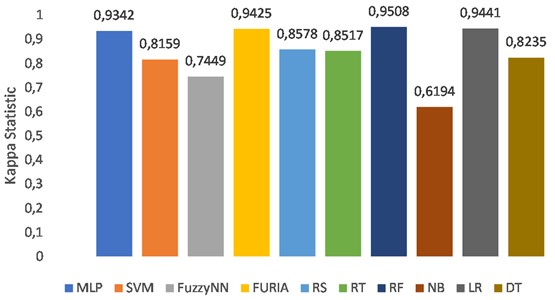
Fig. 5Comparison of the mean absolute error of ten classifiers
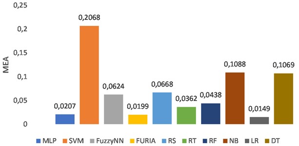
Fig. 6Comparison of the root mean squared error of ten classifiers
4. Conclusions
The study proposed to use machine learning classification methods to estimate the prevalence of obesity in people from Mexico, Peru, and Colombia using accessible data on their eating habits and physical condition. The study highlights the importance of researching the extent of obesity, as it is associated with a wide range of diseases and affects people of all ages and genders. In the study, ten machine learning models – RF, LR, NB, FuzzyNN, SVM, DT, RT, RS, MLP, and FURIA – were used to build an intelligent model for detecting overweight or obese individuals, which can help professionals in the field in their decision-making. The results of the study show that RF achieves the highest accuracy of 95.78 % in performance measures. The study concludes that machine learning is an effective tool in medicine that can be used to make timely treatment decisions for people at risk of obesity.
References
-
“Obesity and overweight.” Word Health organization. https://www.who.int/news-room/fact-sheets/detail/obesity-and-overweight
-
R. Legrand et al., “Commensal Hafnia alvei strain reduces food intake and fat mass in obese mice-a new potential probiotic for appetite and body weight management,” International Journal of Obesity, Vol. 44, No. 5, pp. 1041–1051, May 2020, https://doi.org/10.1038/s41366-019-0515-9
-
K. Prokopidis, E. Chambers, M. Ni Lochlainn, and O. C. Witard, “Mechanisms linking the gut-muscle axis with muscle protein metabolism and anabolic resistance: implications for older adults at risk of sarcopenia,” Frontiers in Physiology, Vol. 12, p. 770455, Oct. 2021, https://doi.org/10.3389/fphys.2021.770455
-
J. Xu et al., “Structural modulation of gut microbiota during alleviation of type 2 diabetes with a Chinese herbal formula,” The ISME Journal, Vol. 9, No. 3, pp. 552–562, Mar. 2015, https://doi.org/10.1038/ismej.2014.177
-
A. T. Wilkins and R. A. Reimer, “Obesity, early life gut microbiota, and antibiotics,” Microorganisms, Vol. 9, No. 2, p. 413, Feb. 2021, https://doi.org/10.3390/microorganisms9020413
-
T. Klancic and R. A. Reimer, “Gut microbiota and obesity: Impact of antibiotics and prebiotics and potential for musculoskeletal health,” Journal of Sport and Health Science, Vol. 9, No. 2, pp. 110–118, Mar. 2020, https://doi.org/10.1016/j.jshs.2019.04.004
-
M. Blüher, “Obesity: global epidemiology and pathogenesis,” Nature Reviews Endocrinology, Vol. 15, No. 5, pp. 288–298, May 2019, https://doi.org/10.1038/s41574-019-0176-8
-
J. Shen, M. S. Obin, and L. Zhao, “The gut microbiota, obesity and insulin resistance,” Molecular Aspects of Medicine, Vol. 34, No. 1, pp. 39–58, Feb. 2013, https://doi.org/10.1016/j.mam.2012.11.001
-
N. Zmora, J. Suez, and E. Elinav, “You are what you eat: diet, health and the gut microbiota,” Nature Reviews Gastroenterology and Hepatology, Vol. 16, No. 1, pp. 35–56, Jan. 2019, https://doi.org/10.1038/s41575-018-0061-2
-
H. Lin, Y. An, F. Hao, Y. Wang, and H. Tang, “Correlations of fecal metabonomic and microbiomic changes induced by high-fat diet in the pre-obesity state,” Scientific Reports, Vol. 6, No. 1, pp. 1–14, Feb. 2016, https://doi.org/10.1038/srep21618
-
D.-H. Kim, D. Jeong, I.-B. Kang, H.-W. Lim, Y. Cho, and K.-H. Seo, “Modulation of the intestinal microbiota of dogs by kefir as a functional dairy product,” Journal of Dairy Science, Vol. 102, No. 5, pp. 3903–3911, May 2019, https://doi.org/10.3168/jds.2018-15639
-
T. Nagano and H. Yano, “Dietary cellulose nanofiber modulates obesity and gut microbiota in high-fat-fed mice,” Bioactive Carbohydrates and Dietary Fibre, Vol. 22, p. 100214, Apr. 2020, https://doi.org/10.1016/j.bcdf.2020.100214
-
T. Nagano and H. Yano, “Effect of dietary cellulose nanofiber and exercise on obesity and gut microbiota in mice fed a high-fat-diet,” Bioscience, Biotechnology, and Biochemistry, Vol. 84, No. 3, pp. 613–620, Mar. 2020, https://doi.org/10.1080/09168451.2019.1690975
-
“About the Body Mass Index (BMI).” National Center for Health Statistics, www.cdc.gov/growthcharts.
-
S. Hiel et al., “Link between gut microbiota and health outcomes in inulin – treated obese patients: Lessons from the Food4Gut multicenter randomized placebo-controlled trial,” Clinical Nutrition, Vol. 39, No. 12, pp. 3618–3628, Dec. 2020, https://doi.org/10.1016/j.clnu.2020.04.005
-
A. Nakamura et al., “Asperuloside Improves Obesity and Type 2 Diabetes through Modulation of Gut Microbiota and Metabolic Signaling,” iScience, Vol. 23, No. 9, p. 101522, Sep. 2020, https://doi.org/10.1016/j.isci.2020.101522
-
Y. Fan and O. Pedersen, “Gut microbiota in human metabolic health and disease,” Nature Reviews Microbiology, Vol. 19, No. 1, pp. 55–71, Jan. 2021, https://doi.org/10.1038/s41579-020-0433-9
-
A. Ballini, S. Scacco, M. Boccellino, L. Santacroce, and R. Arrigoni, “Microbiota and obesity: Where are we now?,” Biology, Vol. 9, No. 12, p. 415, Nov. 2020, https://doi.org/10.3390/biology9120415
-
J. M. Rutkowski, K. E. Davis, and P. E. Scherer, “Mechanisms of obesity and related pathologies: The macro – and microcirculation of adipose tissue,” FEBS Journal, Vol. 276, No. 20, pp. 5738–5746, Oct. 2009, https://doi.org/10.1111/j.1742-4658.2009.07303.x
-
K. W. Degregory et al., “A review of machine learning in obesity,” Obesity Reviews, Vol. 19, No. 5, pp. 668–685, May 2018, https://doi.org/10.1111/obr.12667
-
R. C. Cervantes and U. M. Palacio, “Estimation of obesity levels based on computational intelligence,” Informatics in Medicine Unlocked, Vol. 21, p. 100472, 2020, https://doi.org/10.1016/j.imu.2020.100472
-
E. De-La-Hoz-Correa, F. E. Mendoza-Palechor, A. De-La-Hoz-Manotas, R. C. Morales-Ortega, and S. H. Beatriz Adriana, “Obesity Level Estimation Software based on Decision Trees,” Journal of Computer Science, Vol. 15, No. 1, pp. 67–77, Jan. 2019, https://doi.org/10.3844/jcssp.2019.67.77
-
B. J. Lee, K. H. Kim, B. Ku, J.-S. Jang, and J. Y. Kim, “Prediction of body mass index status from voice signals based on machine learning for automated medical applications,” Artificial Intelligence in Medicine, Vol. 58, No. 1, pp. 51–61, May 2013, https://doi.org/10.1016/j.artmed.2013.02.001
-
X. Pang, C. B. Forrest, F. Lê-Scherban, and A. J. Masino, “Prediction of early childhood obesity with machine learning and electronic health record data,” International Journal of Medical Informatics, Vol. 150, p. 104454, Jun. 2021, https://doi.org/10.1016/j.ijmedinf.2021.104454
-
R. E. Abdel-Aal and A. M. Mangoud, “Modeling obesity using abductive networks,” Computers and Biomedical Research, Vol. 30, No. 6, pp. 451–471, Dec. 1997, https://doi.org/10.1006/cbmr.1997.1460
-
S. A. Thamrin, D. S. Arsyad, H. Kuswanto, A. Lawi, and S. Nasir, “Predicting obesity in adults using machine learning techniques: an analysis of Indonesian basic health research 2018,” Frontiers in Nutrition, Vol. 8, p. 669155, Jun. 2021, https://doi.org/10.3389/fnut.2021.669155
-
S. N. Kumar et al., “Predicting risk of low birth weight offspring from maternal features and blood polycyclic aromatic hydrocarbon concentration,” Reproductive Toxicology, Vol. 94, pp. 92–100, Jun. 2020, https://doi.org/10.1016/j.reprotox.2020.03.009
-
F. M. Palechor and A. L. H. Manotas, “Dataset for estimation of obesity levels based on eating habits and physical condition in individuals from Colombia, Peru and Mexico,” Data in Brief, Vol. 25, p. 104344, Aug. 2019, https://doi.org/10.1016/j.dib.2019.104344
-
“UCI Machine Learning Repository: Estimation of obesity levels based on eating habits and physical condition Data Set.” UCI Machine Learning Repository. https://archive.ics.uci.edu/ml/datasets/estimation+of+obesity+levels+based+on+eating+habits+and+physical+condition+
-
E. Disse et al., “An artificial neural network to predict resting energy expenditure in obesity,” Clinical Nutrition, Vol. 37, No. 5, pp. 1661–1669, Oct. 2018, https://doi.org/10.1016/j.clnu.2017.07.017
-
M. W. Gardner and S. R. Dorling, “Artificial neural networks (the multilayer perceptron)-a review of applications in the atmospheric sciences,” Atmospheric Environment, Vol. 32, No. 14-15, pp. 2627–2636, Aug. 1998, https://doi.org/10.1016/s1352-2310(97)00447-0
-
J. M. Nazzal, I. M. El-Emary, S. A. Najim, and A. Ahliyya, “Multilayer perceptron neural network (mlps) for analyzing the properties of jordan oil shale,” World Applied Sciences Journal, Vol. 5, No. 5, pp. 546–552, 2008.
-
E. Bisong, “The Multilayer Perceptron (MLP),” in Building Machine Learning and Deep Learning Models on Google Cloud Platform, Berkeley, CA: Apress, 2019, pp. 401–405, https://doi.org/10.1007/978-1-4842-4470-8_31
-
L. Auria and R. A. Moro, “Support vector machines (SVM) as a technique for solvency analysis,” SSRN Electronic Journal, 2008, https://doi.org/10.2139/ssrn.1424949
-
N. Cristianini and J. Shawe-Taylor, An Introduction to Support Vector Machines and Other Kernel-based Learning Methods. Cambridge University Press, 2000, https://doi.org/10.1017/cbo9780511801389
-
P. Rivas-Perea, J. Cota-Ruiz, D. G. Chaparro, J. A. P. Venzor, A. Q. Carreón, and J. G. Rosiles, “Support vector machines for regression: a succinct review of large-scale and linear programming formulations,” International Journal of Intelligence Science, Vol. 3, No. 1, pp. 5–14, 2013, https://doi.org/10.4236/ijis.2013.31002
-
J. M. Keller, M. R. Gray, and J. A. Givens, “A fuzzy K-nearest neighbor algorithm,” IEEE Transactions on Systems, Man, and Cybernetics, Vol. SMC-15, No. 4, pp. 580–585, Jul. 1985, https://doi.org/10.1109/tsmc.1985.6313426
-
Miin-Shen Yang and Chien-Hung Chen, “On the edited fuzzy K-nearest neighbor rule,” IEEE Transactions on Systems, Man and Cybernetics, Part B (Cybernetics), Vol. 28, No. 3, pp. 461–466, Jun. 1998, https://doi.org/10.1109/3477.678652
-
M. Dirik, “Implementation of rule-based classifiers for dry bean classification.,” in 5th International Conference on Applied Engineering and Natural Sciences, 2023.
-
J. Hühn and E. Hüllermeier, “FURIA: An algorithm for unordered fuzzy rule induction,” Data Mining and Knowledge Discovery, Vol. 19, No. 3, pp. 293–319, Dec. 2009, https://doi.org/10.1007/s10618-009-0131-8
-
A. Palacios, L. Sánchez, I. Couso, and S. Destercke, “An extension of the FURIA classification algorithm to low quality data through fuzzy rankings and its application to the early diagnosis of dyslexia,” Neurocomputing, Vol. 176, pp. 60–71, Feb. 2016, https://doi.org/10.1016/j.neucom.2014.11.088
-
Z.A. Pawlak, “Rough sets,” International Journal of Computer and Information Sciences, Vol. 11, No. 5, pp. 341–356, Oct. 1982, https://doi.org/10.1007/bf01001956
-
A. Skowron and S. Dutta, “Rough sets: past, present, and future,” Natural Computing, Vol. 17, No. 4, pp. 855–876, Dec. 2018, https://doi.org/10.1007/s11047-018-9700-3
-
Z. Pawlak, “Rough set theory and its applications to data analysis,” Cybernetics and Systems, Vol. 29, No. 7, pp. 661–688, Oct. 1998, https://doi.org/10.1080/019697298125470
-
Zbigniew Suraj, “An introduction to rough set theory and its applications a tutorial,” in ICENCO’2004, 2004.
-
L. Breiman, “Random forests,” Machine Learning, Vol. 45, No. 1, pp. 5–32, 2001, https://doi.org/10.1023/a:1010933404324
-
F. Safarkhani and S. Moro, “Improving the accuracy of predicting bank depositor’s behavior using a decision tree,” Applied Sciences, Vol. 11, No. 19, p. 9016, Sep. 2021, https://doi.org/10.3390/app11199016
-
T. T. Swe, “Analysis of tree based supervised learning algorithms on medical data,” International Journal of Scientific and Research Publications (IJSRP), Vol. 9, No. 4, p. p8817, Apr. 2019, https://doi.org/10.29322/ijsrp.9.04.2019.p8817
-
Gérard Biau, “Analysis of a random forests model,” The Journal of Machine Learning Research, Vol. 13, pp. 1063–1095, Apr. 2012.
-
N. Horning, “Random forests: An algorithm for image classification and generation of continuous fields data sets.,” in International Conference on Geoinformatics for Spatial Infrastructure Development in Earth and Allied Sciences, 2010.
-
D. R. Bellhouse, “The reverend Thomas Bayes, FRS: A biography to celebrate the tercentenary of his birth,” Statistical Science, Vol. 19, No. 1, pp. 3–43, Feb. 2004, https://doi.org/10.1214/088342304000000189
-
P. Domingos and M. Pazzani, “On the optimality of the simple Bayesian classifier under zero-one loss,” Machine Learning, Vol. 29, No. 2/3, pp. 103–130, 1997, https://doi.org/10.1023/a:1007413511361
-
F. Itoo, Meenakshi, and S. Singh, “Comparison and analysis of logistic regression, Naïve Bayes and KNN machine learning algorithms for credit card fraud detection,” International Journal of Information Technology, Vol. 13, No. 4, pp. 1503–1511, Aug. 2021, https://doi.org/10.1007/s41870-020-00430-y
-
E. Frank, L. Trigg, G. Holmes, and I. H. Witten, “Technical note: naive bayes for regression,” Machine Learning, Vol. 41, No. 1, pp. 5–25, 2000, https://doi.org/10.1023/a:1007670802811
-
M. P. Lavalley, “Logistic regression,” Circulation, Vol. 117, No. 18, pp. 2395–2399, May 2008, https://doi.org/10.1161/circulationaha.106.682658
-
M. J. L. F. Cruyff, U. Böckenholt, P. G. M. van der Heijden, and L. E. Frank, “A review of regression procedures for randomized response data, including univariate and multivariate logistic regression, the proportional odds model and item response model, and self-protective responses,” Data Gathering, Analysis and Protection of Privacy Through Randomized Response Techniques: Qualitative and Quantitative Human Traits, Vol. 34, pp. 287–315, 2016, https://doi.org/10.1016/bs.host.2016.01.016
-
B. Kalantar, B. Pradhan, S. A. Naghibi, A. Motevalli, and S. Mansor, “Assessment of the effects of training data selection on the landslide susceptibility mapping: a comparison between support vector machine (SVM), logistic regression (LR) and artificial neural networks (ANN),” Geomatics, Natural Hazards and Risk, Vol. 9, No. 1, pp. 49–69, Jan. 2018, https://doi.org/10.1080/19475705.2017.1407368
-
“Logistic Regression – an overview.” ScienceDirect Topics. https://www.sciencedirect.com/topics/computer-science/logistic-regression
-
R. R. Holland, “Decision Tables,” JAMA, Vol. 233, No. 5, p. 455, Aug. 1975, https://doi.org/10.1001/jama.1975.03260050061028
-
R. Kohavi, “The power of decision tables,” in Lecture Notes in Computer Science, Vol. 912, pp. 174–189, 1995, https://doi.org/10.1007/3-540-59286-5_57
-
D. M. W. Powers, “Evaluation: from precision, recall and F-measure to ROC, Informedness, Markedness and Correlation,” Journal of Machine Learning Technologies, Vol. 2, No. 1, pp. 37–63, 2022.
-
A. Tharwat, “Classification assessment methods,” Applied Computing and Informatics, Vol. 17, No. 1, pp. 168–192, Jan. 2021, https://doi.org/10.1016/j.aci.2018.08.003
-
M. Haggag, M. M. Tantawy, and M. M. S. El-Soudani, “Implementing a deep learning model for intrusion detection on apache spark platform,” IEEE Access, Vol. 8, pp. 163660–163672, 2020, https://doi.org/10.1109/access.2020.3019931
-
D. Chicco and G. Jurman, “The advantages of the Matthews correlation coefficient (MCC) over F1 score and accuracy in binary classification evaluation,” BMC Genomics, Vol. 21, No. 1, pp. 1–13, Dec. 2020, https://doi.org/10.1186/s12864-019-6413-7
-
T. Fawcett, “An introduction to ROC analysis,” Pattern Recognition Letters, Vol. 27, No. 8, pp. 861–874, Jun. 2006, https://doi.org/10.1016/j.patrec.2005.10.010
-
Y. S. Solanki et al., “A hybrid supervised machine learning classifier system for breast cancer prognosis using feature selection and data imbalance handling approaches,” Electronics, Vol. 10, No. 6, p. 699, Mar. 2021, https://doi.org/10.3390/electronics10060699
-
F. A. Almeida et al., “Combining machine learning techniques with Kappa-Kendall indexes for robust hard-cluster assessment in substation pattern recognition,” Electric Power Systems Research, Vol. 206, p. 107778, May 2022, https://doi.org/10.1016/j.epsr.2022.107778
-
M. Mostafaei, H. Javadikia, and L. Naderloo, “Modeling the effects of ultrasound power and reactor dimension on the biodiesel production yield: Comparison of prediction abilities between response surface methodology (RSM) and adaptive neuro-fuzzy inference system (ANFIS),” Energy, Vol. 115, pp. 626–636, Nov. 2016, https://doi.org/10.1016/j.energy.2016.09.028
-
D. Chicco, M. J. Warrens, and G. Jurman, “The coefficient of determination R-squared is more informative than SMAPE, MAE, MAPE, MSE and RMSE in regression analysis evaluation,” PeerJ Computer Science, Vol. 7, p. e623, Jul. 2021, https://doi.org/10.7717/peerj-cs.623
-
T. Chai and R. R. Draxler, “Root mean square error (RMSE) or mean absolute error (MAE)? – Arguments against avoiding RMSE in the literature,” Geoscientific Model Development, Vol. 7, No. 3, pp. 1247–1250, Jun. 2014, https://doi.org/10.5194/gmd-7-1247-2014
-
X. Deng, Q. Liu, Y. Deng, and S. Mahadevan, “An improved method to construct basic probability assignment based on the confusion matrix for classification problem,” Information Sciences, Vol. 340-341, pp. 250–261, May 2016, https://doi.org/10.1016/j.ins.2016.01.033
-
J. Xu, Y. Zhang, and D. Miao, “Three-way confusion matrix for classification: A measure driven view,” Information Sciences, Vol. 507, pp. 772–794, Jan. 2020, https://doi.org/10.1016/j.ins.2019.06.064
About this article

The authors have not disclosed any funding.
The datasets generated during and/or analyzed during the current study are available from the corresponding author on reasonable request.
The authors declare that they have no conflict of interest.
