Abstract
With the aim of enhancing both the ride comfort and the safety of the vehicle, we propose a new type of suspension with an annular vibration-absorbing structure, and establish a 3-DOF 1/4 vehicle model. The structure parameters and time-delay feedback control parameters are determined by particle swarm optimization algorithms, which take the root mean values of body acceleration, suspension dynamic deflection, and tire dynamic displacement as their optimization objectives. We analyze the stability of the suspension control system to ensure the stability of the time-delay control system through the Routh-Hurwitz stability criterion, characteristic root method, and stability switching method. Then, we compare and analyze the response characteristics of conventional suspension, new suspension without time-delay feedback control, and new suspension with time-delay feedback control under simple harmonic excitation and random excitation. The results show that the new suspension with time-delay feedback control has a significant damping effect on the body under the premise of ensuring the stability of the system.
1. Introduction
The vehicle is a complex multi-body system, and the vibration of the engine, the collision between different parts, and the impact of the unevenness of the road can cause the vibration of the vehicle. Severe vibration can have a negative impact on the health of passengers and vehicle components. The suspension system, as the most important vibration-damping component of the vehicle, functions to transmit the forces and moments exerted between the wheels and the body, to cushion the impact on the ground, and to reduce the vibration caused by various dynamic loads, thus ensuring that the vehicle can drive normally [1]. However, suspension is an automotive component that is difficult to achieve the ideal state because it has to take into account both ride comfort and handling stability, but these two properties are contradictory to each other. Nowadays, the research on improving the overall performance of the car and reconciling the contradiction between smoothness and handling stability is mainly focused on two aspects: firstly, designing a good suspension system; secondly, finding the optimal control method.
Rabinow [2], the American National Bureau of Standards, invented the development of magnetorheological fluid materials in 1948, the appearance of new materials provided new ideas and ways for the development of the suspension. American Lord company installed magnetorheological fluid dampers into the car seat suspension system and carried out road tests, and the results showed that the developed car seat damper has a good effect in improving vehicle ride comfort. Researchers at Carnegie Mellon University, USA, applied the parallel structure of magnetorheological dampers and Stewart as a semi-active vibration isolation platform to the suspension system of an off-road vehicle and achieved the desired vibration isolation effect in a real vehicle test study [3]. Hu et al. [4] studied a magnetorheological damper for a vehicle suspension system, as well as designed a switch-fuzzy hybrid control applied to the damping control of a semi-active suspension, and the simulation results showed that the vibration performance of the vehicle under impact excitation was significantly improved. In 1909, Frahm [5] installed an anti-sway tank on the ship by using the power-absorbing technique, which effectively suppressed the ship's sway, and the prototype of the power-absorbing vibration absorber came into being. Zhang et al. [6] compared the effects of suspensions with and without power absorbers on vehicle performance to conclude that suspensions with power absorbers can effectively control body and wheel vibrations in the high-frequency range. In 2001, University of Cambridge scholar Smith [7] creatively proposed the concept of inertia vessel, through the study of the characteristics of inertia vessel components, Smith found that inertia vessels can meet the vibration isolation requirements of suspensions, and then carried out the research work of applying them to vehicle suspensions, exploring a new way to improve the performance of conventional suspensions. In 2018, Li [8] proposed a three-element integrated ISD suspension, improving the cab and body vibration isolation performance effectively. However, these methods to solve vehicle vibration are using vibration damping and vibration isolation devices, without solving the problem from the suspension structure.
In the control process of a suspension system, the execution of the controller, the issuance and acquisition of signals, the response of the actuator, and the movement of the mechanical structure all produce a certain time-delay phenomenon, which is known as time-delay. Inherent time-delay is an unfavorable factor, which affects the stability of the system, deteriorates the system's performance, and even causes chaos and bifurcation. Therefore, it has received a lot of attention from scholars and has been studied in depth.
At the end of the last century, Olgac’s [9], [10] research team proposed to use the amount of time-delay as an active control parameter to exploit the inherent damping property of time-delay for damping control, and by selecting appropriate time-delay feedback control parameters, the vibration of the main system under simple harmonic excitation can be attenuated to zero, thus transforming the time-delay into a favorable factor. Jalili et al. [11] used multiple identical time-delay dynamic absorbers to suppress the vibration of a multi-degree-of-freedom system, simulated and analyzed under a single simple harmonic excitation, with results demonstrating that time-delay feedback control is still desirable. Zhao et al. [12] investigated the damping performance of time-delay nonlinear dynamical vibration absorbers on the main system based on the multiscale method, and the study showed that the acceleration amplitude of the main system was reduced by 90 % with suitable feedback gain coefficients and time-delay values compared to that of the non-linear dynamical vibration absorbers without time-delay. Li et al. [13] studied the damping of LQR control and time-delay feedback control for the whole vehicle, and it was proven that the reasonable selection of time-delay feedback control parameters is more effective than LQR control for the whole vehicle damping. Zhang et al. [14] applied time-delay feedback control to automotive seat damping, obtained the critical time-delay and stability interval of the system by frequency domain scanning method, and simulated the system under simple harmonic excitation and random excitation, which demonstrated that the time-delay power absorber can greatly suppress the vibration response of the seat under either road excitation, effectively improving the ride comfort.
For these issues, this paper proposes a new type of suspension with annular vibration absorbing structure and applies the time-delay feedback control to the new type of suspension, using particle swarm optimization algorithm (PSO) to obtain the parameters of the annular vibration absorbing structure and the time-delay feedback control parameters under different road excitations, furthermore, applying the Routh-Hurwitz stability criterion, the characteristic root method and the stability switching method to obtain the stability interval of the system, as well as perform numerical validation. Finally, we establish the models of conventional suspension (CS), new suspension without time-delay feedback control (PVASS), and new suspension with time-delay feedback control (TDVASS), to compare and analyze the effect of time-delay feedback control on system damping using the above models.
2. A new suspension with an annular vibration-absorbing structure
2.1. The mechanical model
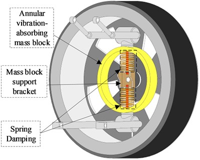
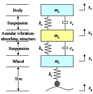
In order to research the effect of the new suspension with the annular vibration-absorbing structure on the body vertical vibration better intuitively, the structure schematic shown in Fig. 1 is constructed, in which the annular vibration-absorbing mass block is connected to the wheel hub and the swing arm support bracket through the spring, damping, and mass block support bracket. For the problem to be researched in this paper, the structure is simplified to a 3-DOF system vibration model including the body, the annular vibration-absorbing structure, and the wheel, as shown in Fig. 2(a). The tire displacement time-delay feedback control is introduced to this model to form the main research object of this paper, as shown in Fig. 2(b), and is analyzed in comparison with the conventional passive suspension, as shown in Fig. 2(c). The physical significance and values of the parameters in the model are shown in Table 1, and due to the small damping of the tires, all the researches in this paper do not consider the tire damping.
Fig. 1A new suspension model with an annular vibration-absorbing structure
Separate the system of degrees of freedom and establish the differential equations of motion of the system according to Newton’s second law:
where, denotes the tire displacement time-delay feedback control force, is the time-delay feedback gain coefficient, and is the time-delay amount.
According to the vehicle suspension performance index and passenger ride comfort performance index, for this purpose, selected body displacement , body velocity , annular vibration-absorbing structure displacement , annular vibration-absorbing structure velocity , tire displacement , tire velocity as state space variables, the differential equation of motion of the system Eq. (1) can be written in the form of the following state space equation:
where, the state variable , ; the input variables , ; the output variable ; and the coefficient matrix of the state-space equation is respectively:
Fig. 21/4 mathematical model
a) PVASS
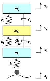
b) TDVASS
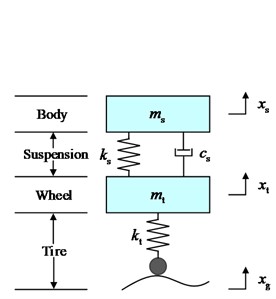
c) CS
2.2. Suspension inherent characteristics analysis
In order to analyze the vibration characteristics of the new suspension system controlled by tire displacement time-delay feedback in the frequency domain, the Fourier transform of Eq. (1) is performed separately to obtain:
which, , ,,, , , , , .
Thus, the frequency response function of the body droop displacement for the pavement excitation displacement input and the amplitude function of the body droop acceleration for the pavement excitation displacement input can be obtained as:
2.3. Annular vibration-absorbing structure parameters determination
The design of new suspension parameters with annular vibration-absorbing structure includes , and . The three parameters have a direct impact on the damping performance of the body. As for the design requirements of the suspension system, one is to achieve compact structure and occupy small space size; the other is to ensure the reliability of all force and moment transmission between the body and the wheels, and to ensure sufficient strength while guaranteeing the mass of components to be small. Therefore, the mass of the annular vibration-absorbing structure is chosen to be 0.1 times the wheel mass , i.e., [15]. The stiffness coefficient and damping coefficient of the annular vibration-absorbing structure were obtained using a particle swarm optimization algorithm [16]. In order to prevent the optimized parameters from not conforming to the actual characteristics of the annular vibration-absorbing structure, the optimization ranges of and were set to and , respectively.
2.3.1. Establishment of the objective function
In this paper, the optimization objective of the new suspension with annular vibration-absorbing structure is to suppress the body vibration to the maximum extent, improve the ride comfort, handling stability and tire grounding of the vehicle, so the RMS values of BA, SDD and TDD are taken as the optimization indexes, and the optimization objective function is established:
where, , , and are weighting coefficients.
2.3.2. Particle swarm optimization algorithm (PSO)
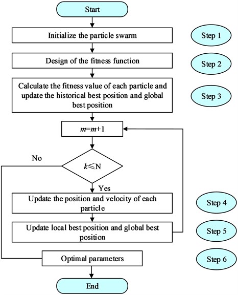
PSO is a classical swarm intelligence algorithm, which mainly uses the sharing of information of individuals in the group, so that the motion of the whole group can produce the evolution process from disorder to order in the problem solution space, and thus obtain the optimal solution of the problem, so the PSO is used to optimize the solution of the stiffness coefficient and damping coefficient of the annular vibration-absorbing structure. The specific steps of the particle swarm optimization algorithm are shown below,
Step 1: Initialize the parameters of the optimization algorithm and generate particles randomly within the parameter optimization range, giving each particle a random initial position and an initial velocity .
Step 2: Design of the fitness function, and in order to optimize the damping performance of the system, the fitness function is therefore designed as shown in Eq. (6).
Step 3: Calculate the fitness value of the generated particles and select the parameter that minimizes the fitness value as the individual best value and the objective function that minimizes the fitness value as the global best value.
Step 4: Update the position and velocity of each particle as shown in Eq. (7):
where is the number of current iterations, is the inertia weight, and are learning factors, and are random values of , is the individual optimal particle position, is the global optimal particle position, is the particle flight speed, and is the current position of the particle.
Step 5: Optimize the second set of parameters, get the individual best and global best according to steps 2 and 3, and compare them with the first set, and update the individual best and the global best.
Step 6: According to the above steps, the individual optimum and the global optimum are updated continuously until the set number of iterations is satisfied, and the system will output the optimized optimum parameters.
The flow chart of the algorithm steps is shown in Fig. 3.
Fig. 3Flow chart of algorithm steps
By the above particle swarm optimization algorithm, the stiffness and damping coefficients of the annular vibration-absorbing structure are optimized, and the optimal parameters of the annular vibration absorbing structure are obtained as 6444 N/m, 348 N⋅s/m. Thus, the vehicle model parameters are shown in Table 1.
Table 1Vehicle model parameters meaning and values
Vehicle parameters | Physical meaning | Values | Units |
Body mass | 345 | kg | |
Annular vibration-absorbing structure mass | 4.05 | kg | |
Wheel mass | 40.5 | kg | |
Vehicle suspension, tire stiffness coefficient | 16000/190000 | N/m | |
Vehicle suspension damping coefficient | 1500 | N⋅s/m | |
Annular vibration-absorbing structure stiffness coefficient | 6444 | N/m | |
Annular vibration-absorbing structure damping coefficient | 348 | N⋅s/m | |
Body, annular vibration-absorbing structure, wheel vertical displacement | – | m | |
Road surface vertical input displacement | – | m |
3. Stability analysis
The selection of time-delay feedback control parameters is decisive for the system to be in a stable state. If the time-delay feedback control parameters are not selected properly, chaos and bifurcation will occur, and in serious cases, the system will be destabilized. In order to ensure that the system is in a stable state, this paper uses the Routh-Hurwitz stability criterion, the characteristic root method and the stability switching method to analyze the stability of the system.
By applying Laplace transform to Eq. (1), the differential equation of motion of the system is deformed into the characteristic equation:
where, is the characteristic root of the equation, and are the coefficients of the polynomial, respectively:
which:
3.1. Time-delay independent stability
Whether the time-delay feedback control can ensure that the system is stable depends on the value of the feedback gain and the time-delay amount . When any value of the time-delay amount is taken, the stability of the system is not changed with the time-delay amount. The stability of the system does not change with the time-delay amount when the time-delay amount takes any value, but only changes with the feedback gain, which is called the full time-delay stable state, i.e., time-delay independent stability. For the time-delay independent stability of the system, it is necessary to satisfy the following two conditions,
(1) When , the characteristic Eq. (8) of the system satisfies Routh-Hurwitz stability.
(2) When , the characteristic Eq. (8) of the system has no positive real roots .
Condition (1): when , the characteristic equation of the system polynomial Eq. (8) is expressed as:
It is concluded from the Routh-Hurwitz stability criterion that for the system to be in a stable state, firstly, all coefficients of the characteristic Eq. (10) of the system are required to be greater than zero; secondly, all terms in the first column of the Routh-Hurwitz table are required to be positive, and the Routh-Hurwitz discriminant table constructed from the polynomial coefficients can be obtained according to Eq. (10), as shown in Fig. 4, which, , , , , , , , , .
Fig. 4Routh-Hurwitz discriminant table
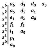
Substituting the parameters of Table 1 into Fig. 4, the stability conditions , , , , , , and can be found to be constant greater than zero. Other stability regions drawn according to the Routh-Hurwitz stability conditions are shown in Fig. 5.
Fig. 5Routh-Hurwitz stability conditions
From Fig. 5, it is clear that when , the polynomial coefficients of the characteristic equation of the system and the first column coefficients in the Routh-Hurwitz discriminant table are greater than zero, which satisfies the Routh-Hurwitz stability criterion and indicates that the no time-delay system is stable in this interval.
Condition (2): When , it is known from stability theory that the asymptotic stability of the time-delay system needs to satisfy that the characteristic roots of the polynomial of the characteristic equation don't contain positive real roots. When the characteristic roots contain pure imaginary numbers, the system is at the boundary of instability and there exists stability switching as well as critical time-delay stability interval. Assuming the existence of imaginary roots in the characteristic equation, the characteristic polynomial of the system Eq. (8) can be expressed as and simplified by using Euler’s formula for , which can be obtained:
where:
Separating the real and imaginary parts shows that if the polynomial Eq. (11) is zero, it must satisfy that both the real and imaginary parts are zero, i.e.:
Further derivation leads to:
With the trigonometric term is eliminated to obtain a polynomial equation for , i.e.:
Such that , the characteristic root discriminant polynomial of the system can be obtained, i.e.:
where:
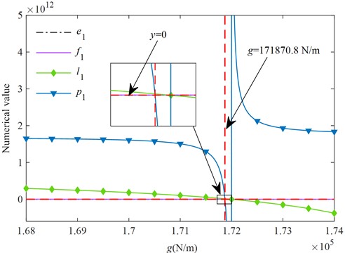
After a series of derivations, can finally be reduced to . By solving the value and number of positive real roots of the polynomial equation , the range of its feedback gain can be determined when the time-delay independent stability is achieved. Fig. 6 shows the time-delay independent stability region of the new suspension under the tire displacement time-delay feedback control.
According to Fig. 6, when , the characteristic equation of the system has no positive real roots, and the range of values of this gain coefficient is in the stability interval of condition Eq. (1), which means that the system is time-delay independent stable in this interval range. When the value range of this feedback gain is exceeded, the polynomial equation has positive real roots, which means that the stability of the system will switch a certain number of times and needs further discussion and analysis.
Fig. 6Time-delay independent stability region
3.2. Stability switching
When the time-delay feedback control parameter is outside the region of time-delay independent stability, the stability of the system is not fixed, and the sign of the real part of the characteristic root changes with time-delay, which means that the stability of the system changes with time-delay, and this situation is called stability switching. Therefore, finding the critical time-delay is crucial to analyze whether the system is stable or not.
Assuming that the polynomial Eq. (15) has positive real roots , all the critical time-delays corresponding to the positive real roots can be solved by the following equation:
where, , .
After all the critical time-delays are determined by Eq. (16), the change of the real part of the characteristic root corresponding to each critical time-delay is then judged to further determine whether the system is stable or not. The characteristic equation polynomial Eq. (8) can be regarded as a function of with respect to . Its derivative can be obtained from the stability switching discriminant formula:
Then, the change of the real part of the characteristic root can be determined according to the positive or negative sign of . In the case of , as the time-delay increases, it means that the real part of the characteristic root crosses the imaginary axis from left to right in the complex plane, thus switching the system from stable to unstable state; in the case of , it means that the real part of the characteristic root crosses the imaginary axis from right to left in the complex plane, and the system switches from unstable to stable state. The following is a concrete example to further illustrate the switching principle of stability.
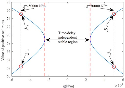
When 50000 Ν/m, the number of positive real roots of the characteristic equation is two, 62.3487, 75.1147, according to Eq. (15), as shown in Fig. 6. Substituting these two positive real roots into Eq. (17), we can get and , and thus the critical time-delay corresponding to these two positive real roots can be found according to Eq. (16) as:
The obtained critical time-delays are sorted to obtain:
Since , i.e., , when the time-delay crosses the time-delay , the real part of the characteristic root changes from positive to negative, and the system switches from unstable to stable state; similarly, when , i.e., , the time-delay crosses , and the real part of the characteristic root changes from negative to positive, then the system switches from stable to unstable state. From the above analysis, it can be seen that when , the system is asymptotically stable; when , the system is unstable. From Eq. (19), it can be seen that the critical time-delay is followed by , no switching occurs, for two consecutive unstable critical time-delays, then it shows that after , the system is always in an unstable state. The final time-delay interval that puts the system in a stable state when 50000 Ν/m is obtained is .
When = –50000 Ν/m, the positive real roots of the characteristic equation are obtained as 62.3487, 75.1147, respectively, as shown in Fig. 6. Further solving for and , then the critical time-delays corresponding to these two positive real roots are obtained as:
The obtained critical time-delays are sorted to obtain:
It can be concluded that no switching occurs after the critical time-delay , which directly becomes , for two consecutive unstable critical time-delays, then it is derived that after the system are in an unstable state. Therefore, when = –50000 N/m, the critical time-delay interval that keeps the system stable is .
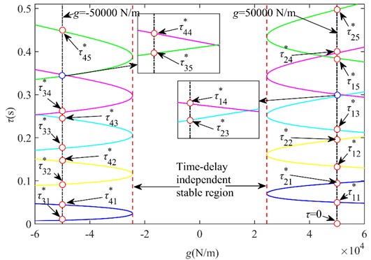
Fig. 7 shows the critical time-delay curves of under tire displacement time-delay feedback control. The intersection of the purple and light blue curves on the right side of Fig. 7 is before the critical time-delay point, and the system is stable, while the intersection of the green and purple curves is after the critical time-delay point, and the system is unstable, and the system state has changed, i.e., the stability switching occurs between shown in the figure. Similarly, the intersection of the purple and light blue curves on the left side of Fig. 7 is on the outside of the critical time-delay point, and the system is stable, while the intersection of the green and purple curves is on the inside of the critical time-delay point, and the system is unstable, which indicates that the system has switched stability between .
Fig. 7(g,τ) critical time-delay curves graph
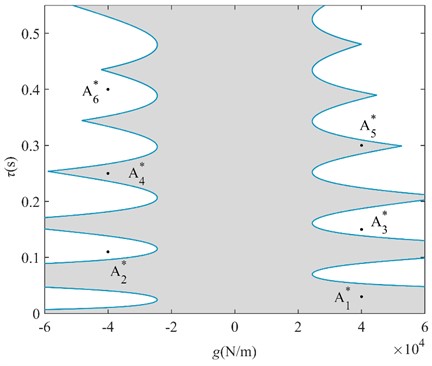
In the case that the gain coefficient is determined, the polynomial solution of the characteristic equation is used to get the positive real roots. If there are no positive real roots in the equation, the system is stable regardless of the value of ; if there are positive real roots in the equation, the system will undergo a certain stability transformation and finally become unstable. According to the change of the number of positive real roots, we can get the full time-delay stability region and stability switching region of the system, and then judge whether the system corresponding to the critical time-delay point is in the stable state according to the stability switching discriminant formula, and finally we can get the critical stability region in the plane under the tire displacement time-delay feedback control, as shown in Fig. 8.
Fig. 8Critical time-delay stability region
3.3. Stability verification
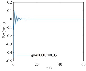
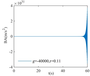
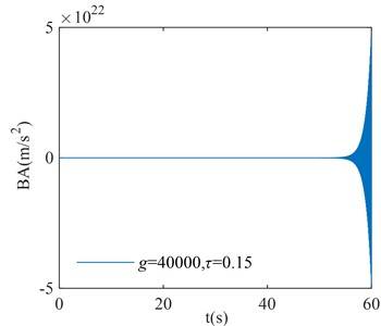
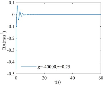
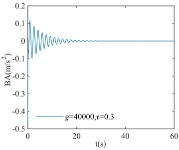
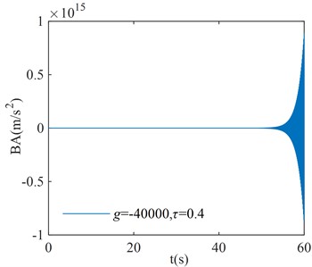
In order to verify the correction of the region in Fig. 8, three points are randomly selected for verification in each stability interval and instability interval of the system, where points (, ), ( –40000, 0.25), and ( 40000, 0.3) correspond to the stability interval of the system; points (–40000, 0.11), ( 40000, 0.15), and ( –40000, 0.4) correspond to the instability interval of the system. The coordinates of each point are substituted into Eq. (1), and the initial condition is taken as . The numerical verification results of the BA at each point are shown in Fig. 9.
Fig. 9Numerical verification results
a)
b)
c)
d)
e)
f)
From the numerical verification results in Fig. 9, it can be seen that when the initial excitation of the system is given, the BA vibration amplitude gradually converges to zero, which indicates that the system is asymptotically stable; the BA vibration amplitude gradually diverges to infinity, which indicates that the system is unstable. The verification results in Fig. 9 are consistent with the corresponding system stability cases in Fig. 8, and the numerical simulation results verify the correctness of the critical stability time-delay stability region map.
4. Solving for optimal time-delay feedback control parameters
4.1. Method of solving the time-delay equation
The solution is difficult because the characteristic equation contains a transcendental function term. Therefore, in this paper, the fine integration method of time-delay differential equations is used to solve the numerical solution of each response quantity of the 1/4 vehicle model vibration.
At first, treating the time-delay feedback control term in Eq. (2) as the excitation term, the solution of the equation can be written as:
Next, the numerical discretization of Eq. (22) is performed by assuming that the simulation time is . Taking the time step , then , the solution of the equation is discretized into the following stepwise integral equation in recursive form:
The above equation can be further derived as:
where, , is expressed as the number of nodal steps that the time-delay quantity is divided into during the solution process. Further solving the solution of Eq. (24), assuming the initial condition of the equation, the system vibration response of each mass block (body, annular vibration-absorbing structure, wheels) at each time point is found as:
where, , represents the vibration displacement response and vibration velocity response of the body mass at time ; , represents the vibration displacement response and vibration velocity response of the annular vibration-absorbing structure mass at time ; , represents the vibration displacement response and vibration velocity response of the tire mass at time , respectively.
Finally, by substituting Eq. (25) into Eq. (1), the vibration acceleration of the body, the annular vibration-absorbing structure and the tire in the time domain are obtained respectively:
4.2. Optimization of feedback control parameters
For the optimization of the time-delay feedback control parameters the PSO described above is still used, and its objective function is shown in Eq. (6). With 100 randomly generated particles and 200 iterations, the fine integration method for solving the time-delay and the pavement displacement are introduced into the PSO to optimize the objective function in the time domain and solve the appropriate time-delay feedback control parameters for different pavements. The simple harmonic excitation and random excitation are selected for the pavement displacement, and the variation curves of the adaptation degree values with the number of iterations for different pavement excitations are shown in Fig. 10. From Fig. 10, it can be seen that the optimal time-delay feedback control parameters are basically obtained at the later stage of the iteration number, and the optimal time-delay feedback control parameters under simple harmonic excitation and random excitation are finally obtained as 5386 N/m, 2×10⁻⁴ s and 2528 N/m, 1.28×10⁻⁴ s, respectively. The optimized two sets of parameters are in the stability region in Fig. 8, which can make the system in a stable state, indicating that the optimized time-delay feedback control parameters are reasonable.
Fig. 10Adaptation function change curves
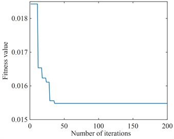
a) Simple harmonic excitation
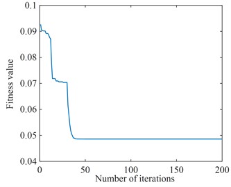
b) Random excitation
5. Simulation results analysis
5.1. Simulation analysis under simple harmonic excitation
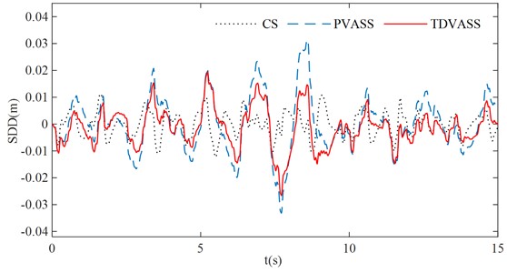
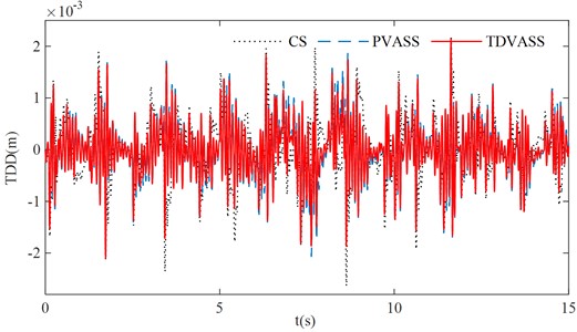
The above optimized tire displacement time-delay feedback control parameters and are substituted into Eq. (1), and the simple harmonic excitation is simulated as the tire road input. The effects of the CS, the PVASS, the TDVASS on the system damping performance in the time domain are analyzed. The simulation curves of each response of the system were obtained as shown in Fig. 11, and the RMS values of each response quantity of the system were shown in Table 2.
As can be seen from Fig. 11, under the optimal feedback control parameters, the BA, SDD and TDD of the TDVASS are reduced compared with the PVASS, and the amplitude is lower in the full frequency domain than that of the PVASS; while compared with the CS, the BA and TDD are significantly reduced, and the SDD compared with the CS, the BA and TDD are significantly reduced, while the SDD is slightly deteriorated, but the increase is still within the design requirement (the suspension dynamic travel of ±100 mm is selected in this paper [17]), which doesn’t exceed the limit travel of the suspension dynamic deflection, i.e., it doesn’t increase the probability of hitting the limit block.
Table 2RMS values of vehicle performance indicators under simple harmonic excitation
RMS values | BA (m/s2) | SDD (m) | TDD (mm) |
CS | 1.6081 | 0.0312 | 3.1109 |
PVASS | 0.9715 | 0.0693 | 1.6606 |
TDVASS | 0.3068 | 0.0388 | 0.6251 |
Fig. 11Simulation comparison under simple harmonic excitation
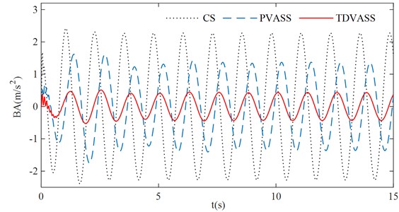
a) Body droop acceleration
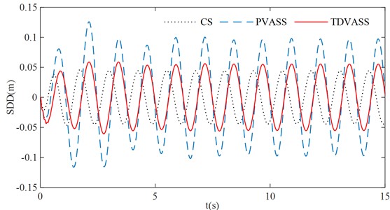
b) Suspension dynamic deflection
c) Tire dynamic displacement
In Table 2, it can be obtained that compared with the CS, the RMS values of BA and TDD of the TDVASS are reduced from 1.6081, 3.1109 to 0.3068, 0.6251, respectively, and the optimization ratios are 80.92 % and 79.91 %; compared with the PVASS, the RMS values of BA, SDD, TDD of the TDVASS are reduced from 0.9715, 0.0693, 1.6606 to 0.3068, 0.0388, 0.6251, respectively, and the optimized ratios are 68.42 %, 44.01 %, 62.36 %, respectively. The above analysis shows that the tire displacement time-delay damping control method can effectively alleviate the impact of road excitation on the body vibration, so that its comfort can be significantly improved. At the same time, the grounding of the tires is also improved, which guarantees the safety of the vehicle.
5.2. Simulation analysis under random excitation
The simple harmonic excitation is only for a certain fixed frequency pavement, which is more desirable for a road, while the random excitation is more in line with the actual road conditions. According to the filtered white noise method described in ISO 8608:1995 as shown in Eq. (27), a standard C-level random road surface [18] is constructed as shown in Fig. 12(a), which is used to further verify the damping effect of the TDVASS on the body. To illustrate the effectiveness of the time domain random pavement excitation model generated based on the filtered white noise method, a comparative power spectral density plot of the C-level pavement is established, as shown in Fig. 12(b), which shows that the simulated power spectral density of the pavement unevenness is in good agreement with the standard power spectral density, indicating the correctness of the generated pavement. This pavement can be used for simulation analysis of the model:
where, is the under cut-off frequency, generally take ; is the A-H level pavement unevenness coefficient; is the reference spatial frequency, 0.1 m-1; is the car driving speed, this paper takes 20 m/s; is the Gaussian white noise signal with zero mean value.
Fig. 12C-level pavement
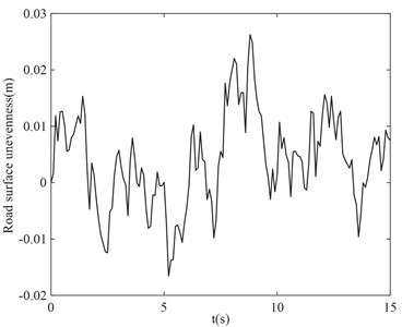
a) C-level pavement unevenness
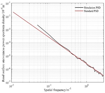
b) Power spectrum density comparison chart
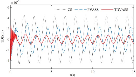
Using Fig. 12 (a) as the random excitation of the pavement and substituting the optimal feedback control parameters and into Eq. (1), the simulation curves of each response quantity of the system are shown in Fig. 13, and the root mean square values of each response quantity of the system are shown in Table 3.
Fig. 13Simulation comparison under random excitation
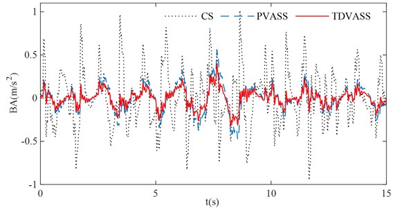
a) Body droop acceleration
b) Suspension dynamic deflection
c) Tire dynamic displacement
Table 3RMS values of vehicle performance indicators under random excitation
RMS values | BA (m/s2) | SDD (m) | TDD (mm) |
CS | 0.3184 | 0.0047 | 0.6399 |
PVASS | 0.1512 | 0.0105 | 0.5607 |
TDVASS | 0.1014 | 0.0073 | 0.5289 |
According to Fig. 13 and Table 3, it can be concluded that the TDVASS has greater advantages compared to the CS and the PVASS. Compared with the CS, the RMS values of BA and TDD are reduced from 0.3184, 0.6399 to 0.1014, 0.5289, respectively, with the optimized ratio of 81.72 % and 19.41 %, and the SDD is slightly deteriorated, but its vibration amplitude is still within the dynamic travel of the suspension and does not exceed its limit travel. Compared with the PVASS, the RMS values of BA, SDD, and TDD were reduced from 0.1512, 0.0105, and 0.5607 to 0.1014, 0.0073, and 0.5289, respectively, with optimization ratios of 61.51 %, 28.57 %, and 8.03 %. As a result, it can be derived that the time-delay feedback control can also effectively reduce the body vibration and improve the comfort of the vehicle and the grounding of the tires under the random excitation with the selection of suitable feedback parameters.
5.3. Amplitude and frequency characteristics analysis
Through frequency domain analysis of CS, PVASS and TDVASS, the response quantities of each vibration characteristic of the suspension system at different frequencies in the studied frequency band can be obtained, and the effect of different time-delay feedback control on vehicle damping can be further investigated. With Eq. (4) and (5), the amplitude frequency characteristic functions of the system can be obtained. The optimal time-delay feedback control parameters and obtained under random road excitation are substituted into the system to obtain the amplitude frequency characteristic curves of BD and BA under tire displacement time-delay feedback, as shown in Fig. 14.
Fig. 14Amplitude frequency characteristic curves
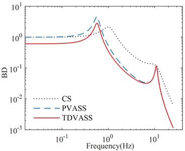
a) Body droop displacement
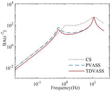
b) Body droop acceleration
It can be seen that due to the addition of the under-spring mass annular vibration-absorbing structure to form the PVASS on the basis of the CS , and the introduction of the tire displacement time-delay feedback control to form the PVASS, which results in the low frequency resonance frequencies of the PVASS and the TDVASS being smaller than those of the CS, and the high frequency resonance frequencies are almost unchanged. It can also be concluded that compared with the CS, the TDVASS only has a certain degree of deterioration in the low frequency resonance region, and the optimization effects in the rest of the frequency bands are substantially improved. With PVASS, the amplitude frequency characteristic curves of BD and BA in TDVASS show substantial improvement in both the low frequency region and the medium frequency region, and the curves almost overlap in the high frequency region with no obvious optimization effect. The above analysis shows that TDVASS has obvious effect on reducing body vibration in the low and medium frequency bands, and the optimization effect is not obvious in the high frequency band.
6. Conclusions
In this paper, a new suspension with an annular vibration absorbing structure is designed to reduce body vibration, and a time-delay feedback control strategy based on tire displacement is introduced to further suppress body droop vibration and improve comfort. The main conclusions are as follows:
1) Designed a new suspension with an annular vibration-absorbing structure, and derived the parameters of the annular vibration-absorbing structure by PSO. And the time-delay feedback control of the tire displacement is introduced, and the parameter values of the time-delay feedback control determine whether the system is stable or not.
2) The time-delay independent stability region of the system is obtained by using the characteristic root method, in which the critical time-delay stability region is obtained by using the stability switching method, meanwhile, the correctness of the stability switching method is verified by numerical simulation.
3) The vibration differential equations of the time-delay system are solved by the fine integration method, and the time-delay feedback control parameters are optimized by introducing the fine integration method and different road excitations into the PSO, and finally the optimal time-delay feedback control parameters for different road surfaces are obtained, so that the system can obtain the best vibration damping control effect.
4) Simulation analysis of the optimal feedback control parameters for different road surface excitation in time domain and frequency domain shows that the tire displacement time-delay feedback control has a significant effect on the body vibration damping. It shows that the time-delay feedback control can significantly improve the ride comfort and tire grounding of the vehicle while ensuring the driving safety.
References
-
T. Wu and H. Hua, Mechanical Vibration. Tsinghua University Press, 2014.
-
J. Rabinow, “The magnetic fluid clutch,” Electrical Engineering, Vol. 67, No. 12, pp. 1167–1167, Dec. 1948, https://doi.org/10.1109/ee.1948.6444497
-
T. Leader and K. Peterson, “Red team too Darpa grand challenge 2005 technical paper,” Carnegie Mellon University, Technical report, 2005.
-
G. Hu, Q. Liu, and G. L., “Hybrid damping fuzzy current control of semi-active vehicle suspension with magnetorheological damper,” Modern Manufacturing Engineering, Vol. 10, pp. 94–101, 2018, https://doi.org/10.16731/j.cnki.1671-3133.2018.10.015
-
U.S. Patent, 989.958, Apr. 1909.
-
X. Zhang, S. Huang, and P. Wu, “Analysis on active suspensions with dynamic absorbers,” Journal of Jiangsu University (Natural Science Edition), Vol. 3, pp. 213–216, 2005, https://doi.org/10.3969/j.issn.1671-7775.2005.03.008
-
M. C. Smith, “Synthesis of mechanical networks: The Inerter,” IEEE Transactions on Automatic Control, Vol. 47, No. 10, pp. 1648–1662, Oct. 2002, https://doi.org/10.1109/tac.2002.803532
-
L. Lei, J. Lei, L. Lin, and J. Zhang, “Integration design and analysis of ISD suspension,” Journal of Guangxi University (Natural Science Edition), Vol. 43, No. 3, pp. 869–879, 2018, https://doi.org/10.13624/j.cnki.issn.1001-7445.2018.0869
-
N. Olgac and B. T. Holm-Hansen, “A novel active vibration absorption technique: Delayed resonator,” Journal of Sound and Vibration, Vol. 176, No. 1, pp. 93–104, Sep. 1994, https://doi.org/10.1006/jsvi.1994.1360
-
N. Olgac and B. Holm-Hansen, “Design considerations for delayed-resonator vibration absorbers,” Journal of Engineering Mechanics, Vol. 121, No. 1, pp. 80–89, Jan. 1995, https://doi.org/10.1061/(asce)0733-9399(1995)121:1(80)
-
N. Jalili and N. Olgac, “Multiple delayed resonator vibration absorbers for multi-degree-of-freedom mechanical structures,” Journal of Sound and Vibration, Vol. 223, No. 4, pp. 567–585, Jun. 1999, https://doi.org/10.1006/jsvi.1998.2105
-
Y. Zhao, “Effect of time-delay feedback control on vibration system damping,” Ph.D. thesis, Tongji University, Shanghai, China, 2007.
-
S. Li, Y. Sun, and J. Liu, “Applications of LQR and time-delayed feedback control in vibration reduction of the vehicle,” Computer Engineering and Software, Vol. 41, No. 2, pp. 12–17, 2020.
-
Y. Zhang, C. Ren, K. Ma, Z. Xu, P. Zhou, and Y. Chen, “Effect of delayed resonator on the vibration reduction performance of vehicle active seat suspension,” Journal of Low Frequency Noise, Vibration and Active Control, Vol. 41, No. 1, pp. 387–404, Mar. 2022, https://doi.org/10.1177/14613484211046458
-
X. Zhang and P. Wu, “Study on suspensions with dynamic absorbers,” Journal of Jiangsu University (Natural Science Edition), Vol. 5, pp. 389–392, 2004, https://doi.org/10.3969/j.issn.1671-7775.2004.05.006
-
L. Chen, D. Shi, H. Jiang, and R. Wang, “A particle swarm algorithm-based parameter optimization method for vehicle suspension systems,” CN103646280A, China, 2013.
-
Y. Qu, “Research on the influences of the active suspension vibration suppression based on the time-delay feedback control,” Shandong University of Technology, Zibo, China, 2016.
-
“ISO 8608-1995, Mechanical Vibration-Road Surface Profiles-Reporting of Measured Data,” International Organization for Standardization, 1995.
About this article

This work was supported by National Natural Science Foundation of China (Grant No. 51275280).
The datasets generated during and/or analyzed during the current study are available from the corresponding author on reasonable request.
Yajie Chen: formal analysis, methodology, software, writing-original draft preparation. Kehui Ma: writing-review and editing. Chuanbo Ren: funding acquisition. Yang Nan: validation. Pengcheng Zhou: validation.
The authors declare that they have no conflict of interest.
