Abstract
A variety of undesired vibrations and noise are usually mixed in high-pressure and sub-high-pressure gas pipeline leak vibration signals. For effectively separating leak vibration signals so that the leak aperture can be identified and localized, an underdetermined blind source separation method is proposed based on the empirical mode decomposition (EMD) and the joint approximate diagonalization of eigenmatrices (JADE). Leak vibration signals were collected by different sensors and then decomposed by the EMD, and multiple intrinsic mode functions (IMFs) were obtained. By calculating the IMF kurtosis values and normalizing them, the characteristic IMFs that contain most of useful leak vibration information were chosen. These characteristic IMFs were reconstructed, and the reconstructed vibration signal and the originally observed signals formed a new matrix. The new observation matrix was used to realize the separation of vibration signals with the JADE algorithm and to solve the underdetermined blind separation problem. Experimental data analysis results show that the proposed method can extract leak signals effectively.
1. Introduction
With the rapid acceleration of economic development and urbanization, natural gas as a clean and green energy source is becoming the preferred energy source that meets the requirements of industries and the urban population. The worldwide natural gas transport and distribution network is complex and continuously expanding. Consequently, natural gas pipelines have formed a transport network covering the entire country. According to studies, pipelines are the safest means of transport of natural gas, but this does not mean that this type of transport is risk free. Pipelines used for transporting natural gas may have small leaks because of some inevitable reasons such as aging, corrosion, and weld defects. The impacts of these leaks extend beyond the costs incurred because of downtime and repair expenses, and can include human injuries as well as environmental disasters. In fact, pipeline leakage has become a major concern and seriously threatens the safe operation of pipelines. Therefore, assuring the reliability of the gas pipeline infrastructure has become a critical need for the energy sector.
The traditional methods based on chemical sensors cannot effectively detect small leaks because of several influencing factors such as a closed pipe trench or air flow along the ground surface. The detection methods widely used in long-distance pipelines, such as negative pressure wave and acoustic wave methods require the sensors to be plugged into the pipeline to detect the leak vibration signals propagating along the medium. These methods either damage the pipeline or cannot ensure combustible gas detection. Therefore, such methods cannot be used to detect leak vibration signals in high-pressure and sub-high pressure gas pipelines [1, 2].
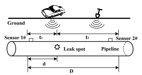
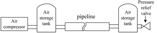
When a leak occurs, there exists impact and friction among the pipeline, air, sands etc and also there involves wall attachment phenomena, Kalman eddy current, edge effect etc. All of these are dynamic and transient and cause the pipeline vibration with different frequencies. So an air-structure coupling is formed between the high-speed escaping gas and the pipeline wall surrounding the leak, thus resulting in a complex vibration signal-stress wave that propagates along the body of the pipeline on both sides of the leak. The stress wave is general acoustic emission signal and on the viewpoint of acoustic the gas pipeline leakage is a pressure field variation process which is induced by the turbulent fluctuation. Studies show the vibration signals of pipelines leak is complicated but the leak process still meets the theory requirement of ideal fluid fluctuation and can be analyzed by the related vibration theory [3, 4]. A mechanical model of impact truing was set up based on the theory of impact dynamics and stress wave spreading, and stress distribution was described accurately. The leak signals can be detected by installing sensors at both ends of pipe walls and picking up the vibration signals. Fig. 1 illustrates the leak detection principle.
Fig. 1Schematic of pipeline leak vibration detection
When a leak signal is acquired, other types of vibration signals (e.g., from ground motion caused by cars, and excavation and construction around the pipeline) are mixed in the data collected by detection systems. These interference vibration signals are generally considered as noises. At present, the denoising process in most researches is usually conducted by using a method such as time-domain filtering, frequency-domain analysis, and wavelet transform to increase the signal-to-noise ratio (SNR). These methods generally consider the acquired signals as a superposition in which a certain characteristic noise is superposed upon the actual leak vibration signal whose strength is higher than that of noise. Nevertheless, in actual measurements, the strength of the interference signal may be greater than that of the actual leak signal, with a severely reduced SNR. The surroundings of high-pressure and sub-high pressure gas pipelines are complex; some factors that influence the detection process of the actual leakage are interference, noise, signals of unknown characteristics, and uncertain collection system parameters. Separating the actual leak vibration signal from observed data to analyze the leakage is a typical blind source separation (BSS) problem. During the acquisition of leak vibrations, external interfering vibrations are coupled to the pipeline wall, contaminating the real leak signals. Therefore, it is very important to study how to effectively separate leak vibrations and interference signals to improve leakage identification and location accuracy.
The leak signal and interference signals are nonstationary, and the traditional processing methods based on stationary assumption cannot separate them very well, whereas BSS can. The BSS method can separate or estimate source signals from observed signals in the case of unknown transmission characteristics, input information, or a small amount of a priori knowledge. The types of interference vibrations are often more than the number of observed signals. This is a type of underdetermined blind source separation (UBSS) problem in which source signals are more than observed signals, and this scenario is common during actual measurements. Considering the above, this paper proposes an underdetermined blind vibration separation method to effectively extract the leak vibration signals of high-pressure gas pipelines. First, the observed signals are decomposed by empirical mode decomposition (EMD) and multiple intrinsic mode functions (IMFs) are obtained. Second, the IMFs’ normalized kurtosis values are calculated and the principal IMFs containing most of the leak information are selected to reconstruct the signal. The new observation signals are now composed of the reconstructed signals and the original observed signals. Finally, vibration signals are effectively separated from the new observation signals using the joint approximate diagonalization of eigenmatrices (JADE) method.
This paper is organized as follows: Section II introduces the summary of the vibration signal BSS model and methods. Section III presents the proposed method, relevant principles, and processing steps in detail. Section IV describes the field experiment and experimental data analysis, and discusses the analysis results and the influencing factors.
2. Problem formulation of blind source separation
Blind source separation recently is widely used in separation and extraction of vibration signals. This novel theory has attracted more and more attention especially in rolling machine, gear box fault diagnosis and other monitoring and processing of machining process [5]. The objective of BSS is to estimate the original signals mixed with interference signals without any prior information about the sources or the mixing process. BSS has been applied in several areas, such as mechanical vibration signals separation, communication, speech, and biomedical engineering.
The standard BSS problem can be formulated as:
where is an unknown -dimensional vector of source signals, and , are mutually independent sources that can be random variables or stochastic processes (time series). is the -dimensional vector of mixed signals observed by sensors, is an × mixing matrix, is the additive noise vector, and the superscript “” denotes the transpose operator.
BSS is aimed at estimating the source signals from the observed mixture of signals without resorting to any a priori information [6]. When the number of source signals equals the number of observed signals (), the mixing process is defined by an evendetermined (i.e., square) matrix and, provided that it is nonsingular, then the underlying sources can be estimated by a linear feed-forward or feedback neural network. If , the mixing process is defined by an overdetermined matrix and, provided that it is full rank, the underlying sources can be estimated by least-squares optimization or linear transformation involving matrix pseudo-inversion. When the number of sources exceeds that of sensors, i.e., , the BSS problem is referred to as UBSS. In such a case, the sources cannot be obtained directly as in the complete BSS case, as the inverse does not exist.
In general, independent component analysis (ICA) is the main method for achieving the BSS. Nonetheless, the algorithm based on ICA is only suitable for the well- or overdetermined case in which the number of sources is equal to or less than that of sensors. In practice, the well- or overdetermined mixture assumption does not always hold. Hence solving the problem of UBSS is necessary. In the underdetermined case, the problem is more difficult than the complete BSS problem [7]. The UBSS problem has recently received considerable attention and various UBSS algorithms have been reported in literature [8]. Most of the existing UBSS algorithms consist of two steps: estimating the mixing matrix and recovering the source signals . In [8] and [9], several methods based on high-order statistics are presented for the estimation of the mixing matrix. As the mixing matrix is not of full column rank in the underdetermined case, the source signals cannot be obtained by multiplying the mixtures by the pseudo-inversion of . This makes recovering the source signals a very challenging task even if the mixing matrix is known.
In order to recover the source signals, most existing UBSS methods assume that the sources are sparse in time domain or other transformation domains such as the time-frequency (TF) domain. In literature [10], some cluster-based TF-UBSS algorithms have been proposed by assuming that there exists at most one active source at any time-frequency point. The sparsity assumption is relaxed in [11-12] to allow the number of active sources at any TF point to be less than the number of sensors. It should be noted that although some signals such as speech signals have some degree of sparsity, majority of actual signals of other types do not possess the sparsity property. Hence it is important to develop UBSS algorithms that do not impose any sparsity constraint on the sources. Some UBSS approaches have been proposed for the blind separation of non-sparse sources in the underdetermined scenario [13-14], and some researchers have tackled this UBSS problem by increasing the number of observed signals, i.e., method of increasing dimension [15]. The following part will discuss the proposed method for extracting the valid leak signal in detail.
3. Proposed method
3.1. Brief description of empirical mode decomposition
EMD, developed by N. E. Huang [16] et al. for adaptive representation of nonstationary signals, can decompose a complicated signal into a number of IMFs according to the local characteristic time scale of the signal. This method has been widely used in vibration signal decomposition and analysis aspects. It is based on three assumptions: (1) the signal has at least two extreme points (maximum and minimum); (2) the characteristic time scale is defined by the time lapse between successive alternations of local maxima and minima of the signal; and (3) if the signal has no extremes but contains inflection points, then it can be differentiated one or more times to reveal the extremes. A signal satisfying such assumptions could be decomposed into a series of IMFs. Each of IMF must satisfy two conditions:
1) In the entire data set, the number of extremes and the number of zero-crossings must be either equal or differ at most by one.
2) At any point, the mean value of the envelope defined by local maxima and the envelope defined by the local minima is zero.
The empirical mode decomposition method is a sifting process. The algorithm operates through six steps:
i) Identification of all the local extremes (maxima and minima) of the series .
ii) Generation of the upper and lower envelopes via cubic spline interpolation among all the maxima and minima, respectively.
iii) Point-by-point averaging of the two envelopes to compute a local mean series .
iv) Subtraction of from the data to obtain an IMF candidate .
v) Checking the properties of :
• If is not an IMF (i.e., it does not satisfy the previously defined properties), replace with and repeat the procedure from Step (i);
• If is an IMF, evaluate the residue .
vi) Repeating the procedure from Steps (i) to (v) by sifting the residual signal. The sifting process ends when the residue satisfies a predefined stopping criterion.
At the end of the decomposition procedure, we get a residue and a collection of IMFs, named . The original can be exactly reconstructed by a linear superposition:
The residue is the mean trend of . The IMFs , ,…, include different frequency bands ranging from high to low. The frequency components contained in each frequency band are different, and they change with the variation of the signal .
These IMFs represent a series of stationary signals with different amplitudes and frequency bands and indicate the intrinsic fluctuation modes. Analyzing the IMFs will provide a wealth of information about original signals.
3.2. IMF kurtosis feature extraction of leak vibration signals
The kurtosis factor is a dimensionless parameter that describes the degree of a spike waveform, and it increases significantly when the signal contains a large number of impact components. When a pipeline leakage occurs, the resulting effect mainly reflects the shock impact of gas-formed turbulent jet on the wall of the leak hole. This type of vibration signal clearly deviates from the normal distribution. The greater the kurtosis factor is, the greater the impact proportion is. Pipeline leakage information is often found in these signals that contain more impact components. Such impacts also stimulate various inherent vibration components of the pipeline and detection equipment in different frequency bands. The IMFs decomposed by EMD include leakage information. The IMFs with greater kurtosis values contain more impact components, and the leakage information is extracted easily from them. In this paper, we propose a principal IMF selection method to choose this type of IMFs, by analyzing IMFs containing the most leak information and reconstruct the leak vibration signal. The use of IMFs will supplement sensor information and realize increasing dimension of observed signals, which is beneficial during the separation of the signals. The extraction steps of characteristic vectors are as follows:
1) EMD is used to decompose the leak vibration signal and obtain several IMFs and a residue as given by Eq. (2).
2) Ignoring the residue, the IMF kurtosis is calculated from Eq. (3). Sometimes, the values are very large; hence, the IMF kurtosis values are adjusted by normalizing for the convenience of further analysis and processing. The normalized kurtosis is computed according to Eq. (4):
where is the order of IMF; and are the th IMF kurtosis and normalized kurtosis, respectively; is the start point and is the amount of sample dots.
3) The normalized kurtosis containing the signal characters are extracted as feature vectors:
The original can be exactly reconstructed by a linear superposition of IMFs. As mentioned above IMFs with greater kurtosis contain more pulse information; therefore, we choose these IMFs to reconstruct the leak signal and acquire further information [17].
3.3. UBSS algorithm based on EMD and JADE
The processing steps of the proposed UBSS algorithm based on EMD and JADE are as follows:
1) Collect dual-channel leak vibration signals as observation signals and express them as and and denoise them;
2) Decompose the denoised signals by EMD and obtain multiple intrinsic mode components from high to low frequencies and a residue as given by Eq. (2);
3) Ignore the residue and calculate the normalized IMF kurtosis as in Eq. (3) and (4). Then choose the IMFs with greater normalized kurtosis as principal IMFs that contain most of the leak vibration signal characteristics;
4) Add the principal intrinsic mode functions and reconstruct vibration signals; afterward, a new set of observation signals is composed of original observed signals and the reconstructed ones. This step achieves the increasing dimension of measurement data and transforms BSS from the underdetermined case to the overdetermined case;
5) Process the newly obtained observation signals with centralization and whitening; then, obtain the whitening matrix and whitened observation signals;
6) Adopt the joint approximate diagonalization of the eigenmatrices algorithm to process the whitened signals and estimate the source vibration signals.
Steps 5) and 6) involve a series of processes and a BSS method based on JADE algorithm proposed by Cardoso [18]. JADE algorithm is based on the construction of a fourth-order cumulant array from the data and joint approximate diagonalization of the eigenmatrix. The main processing steps are described as follows:
Step 1. Form the sample covariance and compute a whitening matrix .
Define the autocorrelation function of the observed signals as:
here, the superscript “” denotes the complex conjugate. We can obtain the eigenvalues and characteristic vectors by eigendecomposition of . Denote ,,…, the largest eigenvalues and , ,…, the corresponding eigenvectors of . The whitening matrix of the free-noise case is:
This means that the whitening matrix is obtained by the autocorrelation matrix of observed vibration signals, i.e., . Superscript denotes the complex conjugate transpose. Then, left multiple the whitening matrix and we obtain the whitening observed signals:
Whitened signals become a “unitary matrix mix” of the source signals.
Step 2. Compute the sample four-order cumulants of the whitened vibration signals and jointly diagonalize the set by a unitary matrix . Then define the cumulant matrices as follows: with any × matrix is associated a “cumulant matrix” denoted by and:
We can find a set of different matrices , and try to make the matrices as diagonal as possible. The diagonality of a matrix can be measured, for example, as the sum of the squares of off-diagonal elements: . Equivalently, because an orthogonal matrix does not change the sum of squares of matrix elements, the minimization of the sum of squares of off-diagonal elements is equivalent to the maximization of the sum of squares of diagonal elements. Thus, we can formulate the following measure:
where denotes the sum of squares of the diagonal. The matrix will be obtained by joint approximate diagonalization of , i.e., by maximization of .
Step 3. Compute the estimation of original vibration signals by .
Fig. 2 illustrates the schematic of the underdetermined blind leak vibration signals separation algorithm based on EMD and JADE.
Fig. 2Flowchart of underdetermined blind vibration signals separation algorithm based on EMD and JADE
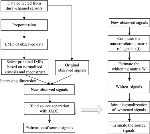
The proposed UBSS method can be summarized in three main steps. First, decompose leak vibration signals observed by EMD and choose principal IMFs to fulfill the increasing-dimension condition; then the underdetermined BSS problem can be transformed into an overdetermined one. The second step is the whitening process that gives rise to the whitening matrix . The third step is joint approximate diagonalization that generates a unitary matrix and estimation of the source vibration signals. The method can process stationary signal separation as well as nonstationary vibration signal separation. Another noteworthy feature is that the method is applicable not only when the number of sources is more than the number of observed signals used for source separation but also when the number of sources is less than that of observed signals.
4. Algorithm verification with simulation signal
4.1. Generation and separation of simulation signals
In this part, a simulation signal was used to verify the proposed algorithm. The simulation source signals included four simulation signals that were mixed by mixing matrix , and then the observation signals were obtained. In this experiment, 3 and 4 i.e. four channels for source signals and two channels for observed signals. The four simulation source signals were generated from a basic formula i.e. Eq. (11):
where , , , and , when 1, 2, 3, 4, these signals were composed of white gaussian noises which means were zero and variances were one were multiplied by 0.5 and then input a FIR low-pass filter. The parameters of the low-pass filter were as follows: order was 21, normalized frequencies were 0.004 and 0.0001. The carrier frequencies were 0.01 Hz, 0.026 Hz, 0.004 Hz, 0.0007 Hz. Using the basic formula can obtain four channel source signals with 3000 sample points. Choose a random mixing matrix , which met the requirement mean was 0 and variance was 1 and obtain the following:
Mixed the source signals with Eq. (1) without noise and then obtained the observed signals. The Fig. 3 showed the source signals and observed signals. The vertical coordinate indicated amplitude of signals and the unite is voltage.
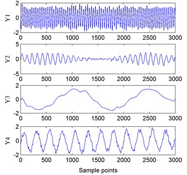
According to the proposed method, the observed signals were decomposed by EMD and Fig. 4 showed the EMD results of observed signals.
Fig. 3Plots of source signals and observed signals
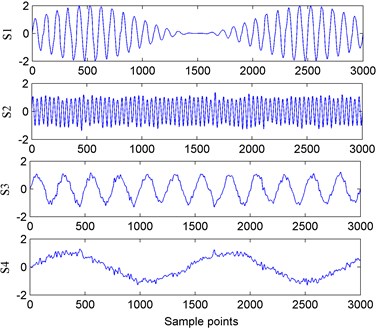
a) Four simulation signals
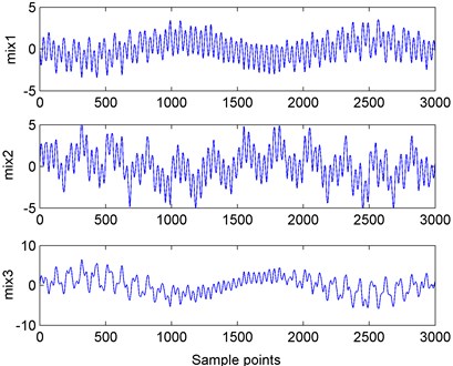
b) Three observed signals
Fig. 4EMD results of three observed signals
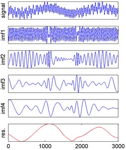
a) EMD result of observed signal 1
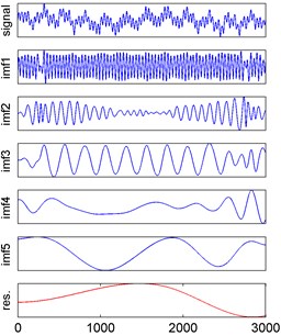
b) EMD result of observed signal 2
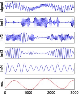
c) EMD result of observed signal 3
The normalized kurtosis values were calculated by Eqs. (3) and (4) and then reconstructed. The Fig. 5 showed the corresponding results.
With the processing steps of proposed method, it can obtain the separated signals and the resulting signal waveforms were shown in Fig. 6. The -axis value indicated the sample dots and -axis value indicated the amplitude of signals and its unit was voltage.
Fig. 5Observed signals IMF normalized kurtosis distributions and reconstructed signals
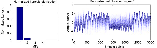
a) IMF normalized kurtosis and reconstructed observed signal 1
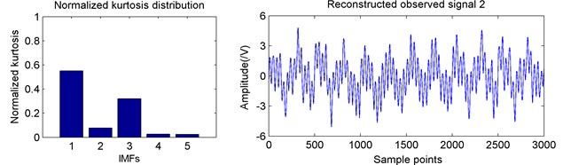
b) IMF normalized kurtosis and reconstructed observed signal 2
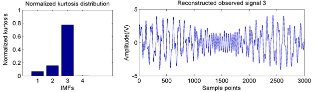
c) IMF normalized kurtosis and reconstructed observed signal 3
Fig. 6Separation results with proposed method
4.2. Evaluation of separation results
This study used the Pearson correlation coefficient as the evaluation index of the separation result. The Pearson correlation coefficient is a statistical index that reflects the degree of correlation between variables. The degree of correlation between two variables is indicated by the multiplication of the deviation. The deviation refers to the difference between a single value and the average. The Pearson correlation coefficient is notated as. The correlation coefficient of two variables and can be expressed as:
where the value of is between –1 and +1, that is, –1 +1. The closer to 1 is, the closer the linear relationship between the two variables is, which indicates that the separated output signal is the estimate of the source signal . If is closer to 0, then is not the estimate of .
According to Eq. (12), the Pearson coefficients of separation results with proposed method were listed in the Table 1.
Table 1Correlation coefficient of separated signals and source signals
Correlation coefficient | ||||
0.0045 | 0.9730 | 0.0175 | –0.0123 | |
–0.9943 | 0.0271 | –0.0248 | –0.0038 | |
–0.0107 | 0.0190 | 0.0173 | 0.9872 | |
0.0117 | 0.0403 | –0.9761 | –0.0186 |
It can be seen from Table 1 that the separated signal was the estimate of the source signal ; was the estimate of , was the estimate of and was the estimate of . The Pearson coefficients indicated that the source vibration signals were well separated by the proposed method.
5. Experiment data acquisition and analysis
5.1. Leak vibration signals acquisition
Considering the safety, cost, and other aspects, the leakage experiment for a pressure pipeline was conducted using air rather than gas (Fig. 7(a)). By using a pressure relief valve, the air flow in the pipeline was maintained at 3.1 m/s. The pressure pipeline used was a seamless steel pipe commonly used in constructing high-pressure pipeline branches. The pipe wall was 4 mm thick, the pipe’s interior diameter was 100 mm, and the length was 100 m. The pressure pipe welding process was used to connect the pipes. Except for the leak part, the pipeline was covered with 20 cm thick sand. In the experiment, we collected vibration signals from three types of sources: the leak, a moving car, and excavation (such as digging). The vibration signals from the latter two sources were considered as the interference signals. The car moved on a rough cement road at 15 to 20 km/h, and the road was 2 to 3 m away from the pipeline. The cement block, which was struck by a splitter to generate vibration, was 5 m away from the leakage hole. Fig. 7(b) showed the layout of pipeline and stimulated interference sources.
The simulated pipeline leak hole was blocked with a ball valve, and the arrangement for the field experiment was shown in Fig. 8. These stimulated leak holes were different apertures that 2 mm, 3 mm, 4 mm and 5 mm, respectively. The pressure gage was used to indicate the pressure in the pipeline.
A piezoelectric sensor was installed as shown in Fig. 9 to collect the vibration signals according to the principle of stress wave propagation.
The components of the vibration signal acquisition system and the relevant parameters were as follows. The piezoelectric sensor with a sensitivity of 0.02 pC/ms-2 and a response frequency range of 0.5 to 20 kHz was selected to collect the vibration signals due to the leak, moving car, and digging. By analyzing the frequency spectrum of these three types of signals, the frequency range of the useful leak vibration signals was found to be between 1 to 8.5 kHz. Then, a piezoelectric sensor with a sensitivity of 4 pC/ms-2 and a response frequency range of 1 to 10 kHz was used to collect the mixed signals. The sampling rate of the data acquisition channel corresponding to each sensor was 50 k sample/second.
Fig. 7Schematic experiment system and layout
a) Schematic of experimental system
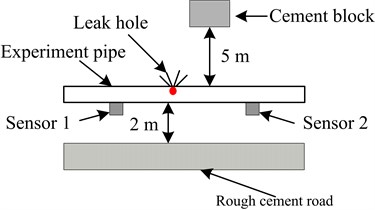
b) Layout of pipeline leak detection sensors and stimulated vibration interferences
Fig. 8Experiment schematic of simulated leaks with different apertures
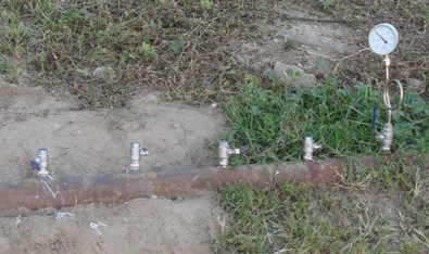
Fig. 9Experimental installation of piezoelectric sensor

5.2. Vibration signals separation and evaluation
In the experiment, the different types of interference signals and stimulated leak vibration signals were first individually collected as the preference source signals and the observation signals were then collected from dual-channel sensors. The time-domain waveforms of the reference vibration source signals of leakage, moving car, and digging that were collected in the experiment were shown in Fig. 10. The -axis value indicated the sample points and -axis value indicated the amplitude of signals and its unit is voltage.
Fig. 11 showed the dual-channel mixed signals of the leak, moving car, and digging obtained by the vibration signal acquisition modules in the same environment. The -axis value indicated the sample dots and -axis value indicated the amplitude of signals and its unit was voltage.
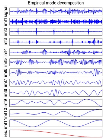
After preprocessing the experimental signal, EMD was used to decompose the vibration signals collected by Sensors 1 and 2, respectively. The EMD decomposition results for Sensor 1 were shown in Fig. 12. The “res” in the figure denoted the residual component.
These IMF components were different from each other. The IMFs’ normalized kurtosis values were calculated and analyzed and then principal IMF components were chosen for reconstruction. Fig. 13(a) shows the IMFs’ normalized kurtosis characteristics corresponding to the signals collected by sensors shown in Fig. 11. From the processing results, most features of Sensor 1 signal were contained in IMF4 and IMF5. The normalized kurtosis of IMF4 accounted for more than 80 % of total kurtosis, and the sum of normalized kurtosis of IMF4 and IMF5 accounted for more than 95 %. The features of Sensor 2 were mainly contained in IMF3-IMF5. After analysis, the principal characteristic vectors selected in this study were IMF4 and IMF5 of Sensor 1 and IMF3-IMF5 of Sensor 2. The reconstructed vibration signal waveforms of Sensors 1 and 2 were shown in Fig. 13(b).
Fig. 10Time-domain waveform of three reference vibration signals
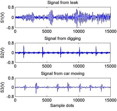
Fig. 11Waveforms of signals acquired from dual channel sensors
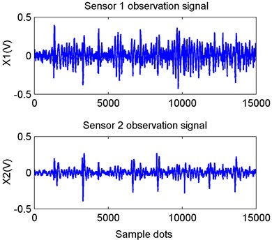
Fig. 12EMD decomposition results for Sensor 1 vibration signal
The originally observed signals and the reconstructed vibration signals comprised the new observation signals. The new observation signals were separated with the JADE algorithm, and the resulting signal waveforms are shown in Fig. 14. The -axis value indicated the sample dots and -axis value indicated the amplitude of signals and its unit was voltage.
By comparing the results in Fig. 10 and Fig. 14, it can be readily seen that the time-domain waveforms of the three separated vibration signals as shown in Fig. 10 were essentially the same as the source signals shown in Fig. 14, and that the leak vibration signal was well separated. Compared with the source signals in Fig. 10, the amplitudes of the three separated vibration signals in Fig. 14 changed and the orders of separated results were not consistent with that of the source signals. This was mainly due to the two uncertainties involved in BSS.
Fig. 13Normalized kurtosis and reconstructed vibration signals of dual-channel sensors
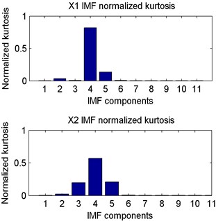
a) Normalized kurtosis of observation vibration signals
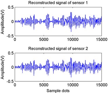
b) Reconstructed signals of dual-channel sensors
The separated vibration signals , , and were compared with source signals , , and . Eq. (12) was used to calculate the correlation coefficient of separation signals and source signals. Table 2 listed the results.
It can be seen from Table 2 that the separated signal was the estimate of the source signal ; was the estimate of and was the estimate of . The Pearson coefficients indicated that the source vibration signals were well separated by the proposed method.
Fig. 14Estimated source vibration signals
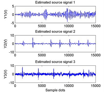
Table 2Correlation coefficient of separated signals and source signals
Correlation coefficient | |||
0.9365 | 0.0696 | 0.0064 | |
0.1211 | –0.0291 | 0.9970 | |
0.0434 | 0.8140 | 0.0315 |
The processing result of the acquisition signals of dual-channel sensors used in the experiment indicated that using EMD and the reconstruction according to IMFs’ kurtosis characteristics, the proposed method realized the increased dimension of the observed vibration signals and changed UBSS to the positive definite or overdetermined case. Additionally, the method could also mine information deeply hidden in the leak vibration signal, to obtain the characteristics of the leak vibration signal. It can be seen from Fig. 10 and Fig. 14 that although there were some errors in the separation results, the total separation effect was relatively satisfactory.
6. Conclusions
This paper proposed a UBSS method to effectively extract the leak vibration signals from a gas pipeline by utilizing the advantages of EMD and JADE. Through analysis and processing of EMD results, the underdetermined blind vibration source separation problem was solved by converting the underdetermined case to an overdetermined case. Experimental results show that this method can effectively separate the mixed signals and extract the leak vibration signal. As the method can be applied to source separation when source signals are more than observation signals as well as when source signals are fewer than observation signals, the proposed method is of great significance to the development of actual pipeline leak signal extraction.
The digging or traffic vibration signals stimulated in this study were some of the known artificial interference sources for which good separation results were obtained in the experiment. However, the efficacy of this method was not satisfactory when separating the interference vibration signals that cannot be modeled by a uniform law because of various unpredictable factors. Identifying and removing such interference vibration signals and extracting the signals produced by a pipeline leakage rapidly and effectively were still key issues that we will study in the future.
References
-
Shin Yong Woo, Kim Min Soo, Lee Sang Kwon Identification of acoustic wave propagation in a duct line and its application of impact source location based on signal processing. Journal of Mechanical Science and Technology, Vol. 24, Issue 12, 2010, p. 2401-2411.
-
Jiedi Sun, Qiyang Xiao, Jiangtao Wen, Fei Wang Natural gas pipeline small leakage feature extraction and recognition based on LMD envelope spectrum entropy and SVM. Measurement, Vol. 55, Issue 9, 2014, p. 434-443.
-
Jin H., Zhang L., Liang W., Ding Q. Integrated leakage detection and localization model for gas pipelines based on the acoustic wave method. Journal of Loss Prevention in the Process Industries, Vol. 27, Issue 1, 2012, p. 74-88.
-
Mostafapour A., Davoudi S. Analysis of leakage in high pressure pipe using acoustic emission method. Applied Acoustics, Vol. 74, Issue 3, 2013, p. 335-342.
-
Li Zhixiong, Yan Xinping, Tian Zhe, et al. Blind vibration component separation and nonlinear feature extraction applied to the nonstationary vibration signals for the gearbox multi-fault diagnosis. Measurement, Vol. 46, Issue 6, 2013, p. 259-271.
-
Peng Dezhong, Xiang Yong Underdetermined blind separation of non-sparse sources using spatial time-frequency distributions. Digital Signal Processing, Vol. 20, Issue 2, 2010, p. 581-596.
-
Lu Fengbo, Huang Zhitao, Jiang Wenli Underdetermined blind separation of non-disjoint signals in time-frequency domain based on matrix diagonalization. Signal Processing, Vol. 91, Issue 7, 2011, p. 1568-1577.
-
Ferreol A., Albera L., Chevalier P. Fourth-order blind identification of underdetermined mixtures of sources (FOBIUM). IEEE Transactions on Signal Processing, Vol. 53, Issue 5, 2005, p. 1640-1653.
-
De Lathauwer Lieven, Castaing Joséphine, Cardoso Jean-Francois Fourth-order cumulant-based blind identification of underdetermined mixtures. IEEE Transactions on Signal Processing, Vol. 55, Issue 6, 2007, p. 2965-2973.
-
Nguyen Linh-Trung, Belouchrani Adel, Abed-Meraim Karim, Boashash Boualem Separating more sources than sensors using time-frequency distributions. EURASIP Journal on Applied Signal Processing, Vol. 2005, 2005, p. 2828-2847.
-
Peng D., Xiang Y. Underdetermined blind source separation based on relaxed sparsity condition of sources. IEEE Transactions on Signal Processing, Vol. 57, Issue 2, 2009, p. 809-814.
-
Aissa-El-Bey A., Linh-Trung N., Abed-Meraim K., Belouchrain A., Grenier Y. Underdetermined blind separation of nondisjoint sources in the time-frequency domain. IEEE Transactions on Signal Processing, Vol. 55, Issue 3, 2007, p. 897-907.
-
Li Y., Wang J. Sequential blind extraction of instantaneous mixed source. IEEE Transactions on Signal Processing, Vol. 50, Issue 5, 2002, p. 997-1006.
-
Thomas J., Deville Y., Hosseini S. Differential fast fixed-point algorithms for underdetermined instantaneous and convolutive partial blind source separation. IEEE Transactions on Signal Processing, Vol. 55, Issue 7, 2007, p. 3717-3729.
-
Li Zhinong, Liu Weibing, Yi Xiaobing Underdetermined blind source method of machine faults based on local mean decomposition. Journal of Mechanical Engineering, Vol. 47, Issue 7, 2011, p. 97-102.
-
Huang N. E., Shen Z., Long S. R., Wu M. C., Shih H. H., Zheng Q., Yen N.-C., Tung C. C., Liu H. H. The empirical mode decomposition and the Hilbert spectrum for nonlinear and non-stationary time series analysis. Proceedings A of the Royal Society, Vol. 454, 1998, p. 903-995.
-
Sun Jiedi, Wen Jiangtao Target location method for pipeline pre-warning system based on HHT and time difference of arrival. Measurement, Vol. 46, Issue 8, 2013, p. 2716-2725.
-
Cardoso J. F., Souloumiac A. Blind beamforming for non-Gaussian signals. IEE Proceedings on Radar and Signal Processing, Vol. 140, Issue 6, 1993, p. 362-370.
About this article
The Project Supported by National Natural Science Foundation of China No. 51204145 and Natural Science Foundation of Hebei Province of China No. E2013203300. The authors offer sincere gratitude to Fei Wang, Ge Guo and the other fellows of China Petroleum and Gas Pipeline Telecommunication and Electricity Engineering Corporation.
