Abstract
Feature mode decomposition (FMD) has advantages over the other newer time-frequency methods such as ensemble empirical mode decomposition (EEMD) and variational mode decomposition (VMD) in single channel blind source separation (SCBSS). However, FMD has the defect of needing to determine the precise number of fault sources manually. To solve the above defect of FMD, an adaptive method for determining the number of fault sources based on the shift invariant sparse code (SISC) is proposed. SISC was used to train a set of basis functions from the single channel signal, and the corresponding potential components were reconstructed firstly. Subsequently, the structural similarity of these potential components was used for clustering, and each of the obtained clustering signals represented one kind of fault. Then the number of clustering was determined by minimizing the structural correlation among the clustering signals. It was considered that the source separation had achieved the best effect when the structural difference among the clusters was the largest, and the number of clustering at this time was used as the optimal estimated value, which was used as the modal inputs number of FMD calculation model to realize SCBSS of rolling bearing. Simulation and experimental analysis were carried out to verify the effectiveness of the proposed method, and its superiority was also verified through comparison.
1. Introduction
As the most common used key supporting component in rotating machinery, the safe running of rolling element bearing is very important. In recent years, amounts of studies relating to rolling bearing have been arising, which include dynamics, [1-3] simulation, [4-5] vibration monitoring [6-7] and fault detection based on self-learning artificial intelligent techniques [8]. As one research branch of fault diagnosis for rolling bearings, the extreme case of underdetermined blind source separation (UBSS) is to separate each source signal from a single channel of observed signal, which has important engineering and implications: 1) The structure of mechanical equipment is often compact, which brings great changes to the installation of sensors. Meanwhile, multiple sensors also cause more cost and maintenance work, so it is more convenient and popular to have as few sensors as possible in engineering application. Even in some cases, only a single sensor can be installed due to space constraints, etc. 2) Even in the case of multiple sensors, it is of great value for subsequent analysis by doing as much analysis and mining as possible on each sensor signal. SCBSS has achieved fruitful research results in speech, signal processing and other signal processing fields [9-11]. Though kinds of studies relating to the problem of UBSS based on multi-channels have been proposed in the area of fault diagnosis, [12-13] there are few researches on SCBSS, [14] and the related research needs to be further deepened.
There are two main problems that needs to be solved as for the application research of SCBSS in fault diagnosis: 1) Separate the observed signal being collected from one single channel sensor into multiple single-component signals to represent each fault source signal effectively. 2) Estimate the number of fault sources correctly. The time-frequency (TF) decomposition method is used widely in solving SCBSS. Usually, the original single-channel observed signal is decomposed into several single components, and then some criteria are constructed according to the obtained single components to estimate the optimal number of fault sources. The Bayesian information criterion of VMD is used to estimate the number of fault sources, and the mixing matrix is estimated by the constructed VMD hyperplane normal vectors [15]. EEMD and constrained independent component analysis (CICA) are combined in UBSS, and sufficient observation signals could be obtained through decomposing the original observation signals by using EEMD. Subsequently, CICA is proposed to retrieve specified source by using kurtosis and waveform factor as constraints [16]. VMD is incorporated into convolutive BSS and a multi-dimensional VMD method is developed and used for bearing crack detection [17]. The bounded component analysis (BCA) is introduced to identify relevant information and a new supervised order tracking BCA is presented for UBSS the fault signals of gear crack [18]. The synchrosqueezing transform is combined with an improved density peak cluster method for solving UBSS problem, and it is verified that this method has good source recovery performance even in the noisy environment [19]. A VMD method guided by fault information is proposed and used to decompose the original multi-components signal of rolling bearing, and satisfactory UBSS results are obtained [20]. VMD is combined with independent component analysis for UBSS of the compound fault of bearings: a series of intrinsic mode functions are obtained by applying VMD on the original signal, and then the demodulated signal is transformed into these multi-channel functions by using Hilbert transform as the input matrix of independent component analysis [21]. However, there existed two defects in the above methods: 1) there are often existing mode mixing phenomenon in most of the above TF methods. 2) The constructed criterions in the above methods often usually assume that there is no existing mode mixing among the decomposed modes, so the constructed criterions are not reasonable to some extent. As a new TF method, FMD considers both the impulsiveness and periodicity of the fault signal, [22] and could remove redundant and mixed modes adaptively during the decomposition process. So FMD is used in the paper as an alternative to traditional TF analysis methods.
As an adaptive and efficient signal processing technology, sparse decomposition has been used widely in fault diagnosis, and most of them mainly focused on weak or compound fault diagnosis of rotating machinery [23-24]. The references relating to the application of sparse decomposition on BSS or UBSS is relative very few. Sparse component analysis (SCA) is the classical sparse decomposition theory-based method for solving the problem of UBSS [25]. The rank and sparsity of signals are used in UBSS of the composite signals of bearing [26]. Furthermore, most of the above references use sparse decomposition for feature extraction or BSS, and very few references studying on the application of sparse decomposition in determining the number of fault sources have been arising. This paper proposes a method for determining the number of fault sources of single channel based on a sparse representation self-learning dictionary.
A SCBSS method for bearing fault diagnosis by combining SISC and FMD is proposed in the paper based on the above stated, and its main contributions are as follows: 1) A fault sources number determination method based on SISC is proposed, which could determine the number of fault sources correctly based only on one single channel observed signal. 2) FMD is used for solving the UBSS problem of bearing fault diagnosis effectively, which has advantage compared with EEMD, VMD and other related TF methods. 3) The proposed method is applied to the compound fault diagnosis of bearing successfully. The remains of the paper are organized as follows: section 1 is dedicated to the fault sources determination method. Flow chart of the proposed method and its details are given in section 2. Section 3 and section 4 are the simulation and experiment verification respectively. Section 5 makes a comparison and section 6 draws a conclusion.
2. Single channel blind source separation based on SISC and self-adaptive clustering
2.1. Single channel blind source separation and SISC model
It is feasible to study the fault state directly through the waveform performance of the signal in case of unpredictable transmission paths from the perspective of diagnosis. Therefore, the linear mixed model is considered and used for single channel BSS in the paper, which is also practical for processing of fault signal. Each source signal could be represented as linear mixture of a set of time-domain features, and the observed signal is linear mixture of these source signals. The single source signal could be expressed as following:
where is the th source signal, is the index set of all the time-domain features corresponding to the source signal . is the coefficients of time domain features. The observed signal is obtained through the linear mixture of source signals:
in which is the gaussian noise. The time-domain features could appear at any time-shifted position in the time series. If is defined as a time-domain feature that appears from the starting position of the observed signal, the time-shift feature representing the non-zero elements in time-domain features could be obtained, and represents the length of the non-zero sub-vectors in the corresponding time domain features. The source signal could then be expressed as one kind of shift-invariant linear mixture:
where is the set of all possible feature time-shifted positions. The observed signal could be expressed as following:
The matrix form of Eq. (4) is as following:
As for the problem of single-channel blind source separation, all the time domain features , the coefficients of and the index set need to be solved, and the solving steps are as following: 1) Obtain through feature self-learning based on the observed signal. 2) Calculate using coefficient solving algorithm. It should be noted that the solving frameworks of both and are under the condition of sparse constraints. 3) Finally, these time domain features are classified by clustering method to obtain the index set of each source signal.
In order to make connections with SISC, we redefine as following:
where , , and can time-shift to any position within the signal. Considering the more general case, let , be one of the single channel observed signals, and Eq. (4) is changed as following:
The Eq. (7) is exactly the expression of the SISC model, and the solving of time-domain features and coefficients based on sparse constraints could be expressed as following:
where , .
It could be seen that the solution of time-domain features and coefficients in the single-channel observation signal could be converted into the solution of basis functions and sparse coefficients in the SISC model, and it is believed that this sparsity constraint is reasonable for solving time-domain features with the observed signal. The process of signal sparse representation is also a process that trends to reveal the intrinsic shape of the signal. The self-learning characteristics of the basis functions are used to solve the time-domain features of the observed signal based on the idea of SISC, so that these time-domain features also tend to converge to the intrinsic shape of the signal. The solution algorithms of coefficient and basis function based on SISC could be referred to reference, [27] which would not be repeated here.
2.2. Self-adaptive clustering
The determination of the time domain feature index set is the key step of source separation, which determines the number of source signals. Refer to the feature self-learning process of SISC, the th basis function (time domain feature) and its coefficient are obtained. Meanwhile, the latent component of the observed signal is also obtained. The th source signal could be reconstructed as following when is determined:
Because the time domain features belonging to the same type of source signal have similar signal structures, so the reconstructed latent components based on them also have similar signal structures. Therefore, the idea of this paper is to determine the index set by the structural similarity between each latent component. There are many ways to characterize the structure of a signal, including the time-domain waveform, frequency spectrum, and envelope spectrum (ES), etc. Although the time-domain waveforms of potential components belonging to different source signals must be different, the potential components of the same source signal may have differences in time-domain waveforms due to different energy or matching to different parts of the source signal. Spectrum is also not the best way to distinguish the structure, because there is likely to have frequency aliasing or similar spectral structure between different source signals. The envelope of the signal also has detailed differences in homologous latent components, which is same as time-domain waveform. The envelope spectrum is essentially one kind of description of the signal envelope, so it is not easily affected by the local detailed differences of the homologous potential components, while the differences of the non-homologous potential components will be clearly reflected in the envelope spectrum. Therefore, we use the envelope spectrum commonly as the index of the similarities and differences of the potential component structure, and we also use the commonly used K-means clustering algorithm as the classification algorithm.
Regarding the optimal number of clustering, kind of estimation methods have been proposed, [31] most of which are based on the idea of minimizing the intro-class distance and maximizing the inter-class distance. However, it is difficult to apply the above methods on the source clustering of fault signals directly. Although the methods are proposed from a general point of view, they do not fully utilize the characteristics of signal processing in fault diagnosis. The optimal clustering number determination method proposed in this paper is based on minimizing the correlation of the envelope spectrum of each source signal, and the calculation equation of the Pearson correlation coefficient of signal and is as following:
where and are the average values of and respectively, and are the standard deviations of and . is a statistical indicator that measures the degree of correlation between two variables, which ranges from +1 to –1. +1 means that the two variables are completely positively correlated, 0 means that they are completely uncorrelated, and –1 means that they are completely negatively correlated. For each possible number of clustering , the index set could be obtained by the above- mentioned K-means clustering of the potential component’ envelope spectrum, and then the source signal could be obtained by using Eq. (10). Eq. (11) is used to calculate the Pearson correlation coefficient between two signals, so the mean value of all the Person correlation coefficients could be calculated simultaneously. The corresponding number of clustering is the optimal estimation of the number clustering when is minimum, because the correlation between the source signals is weakest among all possibilities.
3. Flow chart of the proposed method
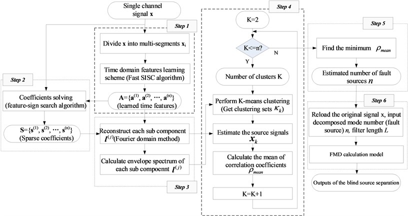
Flow chart of the proposed method is presented in Fig. 1, and its details are as follows:
Step 1: The single channel observed signal is segmented into , so that all the time domain features of the observed signal could be obtained by feature self-learning method, that is, SISC. It should be noted that the number of basis functions in the SISC algorithm should be appropriately large here.
Step 2: The sparse coefficient corresponding to is calculated by sparse coefficient solution according to the results obtained in step 1.
Step 3: Calculate the latent component according to and . Besides, the normalized envelope spectrum of is also calculated.
Step 4: Carry out K-Means clustering using the normalized envelope spectrum of to get the time domain feature index set , and the number of clustering range from 2 to ( is the number of basis functions). Subsequently, reconstruct the latent components according to to get the current source signal , and then the mean of the Pearson correlation coefficient is calculated.
Step 5: Find the smallest after completing all the loops in step 4, and the corresponding number of clustering is determined.
Step 6: Determine the optimal number of patterns for FMD, that is the obtained number of clustering in step 5. Input and other default parameters same as reference [22] into the calculation model of FMD, and then extract the fault features of the output FMD by using envelope spectrum.
Fig. 1Flow chart of the proposed method
4. Simulation
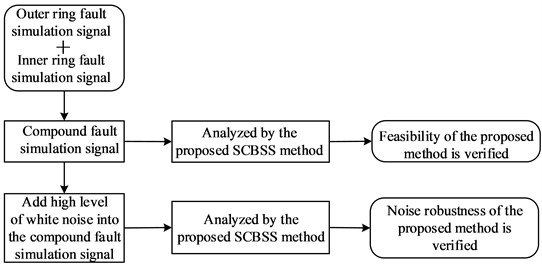
The main flow chart of the simulation is as shown in Fig. 2.
Fig. 2Main flow chart of the simulation
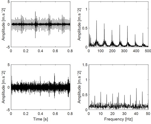
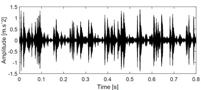
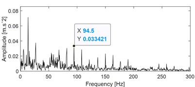
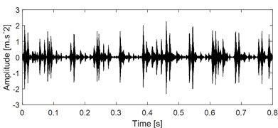
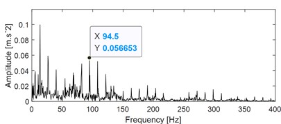
The simulated signal model of failed bearing is shown in Eq. (12), and the outer ring fault and the inner ring fault of bearing are simulated by using Eq. (12). The sampling frequency of the two simulated signals is set as = 265.6 kHz, and the inner ring fault characteristic frequency (FCF) is set as 105 Hz, and the rotating frequency is set as 10 Hz. The outer ring FCF is set as 32 Hz. The compound fault signal of rolling bearing is expressed as the time domain sum of the above two simulated signals. Fig. 3(a) shows the time domain waveforms of the composite signal and its two components (Inner, Outer and Mixed represent the simulated inner ring, outer ring and composite fault signal respectively), and their corresponding envelope spectrum analysis results are given in Fig. 3(b). According to the flow chart of the proposed method shown in Fig. 1, the compound fault signal is segmented firstly: the signal segment length is set to 1024 points, the overlap rate is 0.5, and the basis function length (time domain feature) is 256 points. It should be noted that the compound fault situation is considered here, so the number of basis functions () needs to be appropriately large, which is selected as 8:
Fig. 3Simulated signals of faulty rolling bearing in different running states
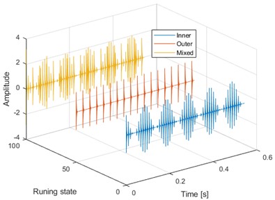
a) Time-domain waveforms of the three simulated signals

b) Envelope spectrum (ES) results of the signals as shown in Fig. 3(a)
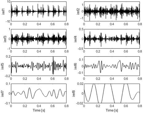
Fig. 4Learned time features and latent components of the mixed signal as shown in Fig. 3(a)
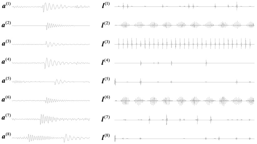
The time domain features ~ and the corresponding latent components ~ as shown in Fig. 4 are obtained finally through the SISC feature learning. It could be observed based on Fig. 4 that the time domain features capture various morphological characteristics buried in the compound signal. Calculate the normalized envelope spectrum of each latent component according to step for K-Means clustering. Then calculate the average of the Pearson correlation coefficient for each possible number of clusters from 2 to , and the relationship between and the number of clusters is shown in Fig. 5, thus it is concluded that when the cluster number is 2, the cluster number is the minimum, so the optimal number of cluster is estimated to be 2, that is, the number of fault source is 2. Then based on step 6 as presented in Fig. 1, the FMD analysis of the original compound fault signal is carried out by using the optimal number of fault sources, and the final analysis result is shown in Fig. 6, and satisfactory fault characteristics are obtained.
Fig. 5The mean value of correlation coefficients for each clustering number (Simulated signal without noise)
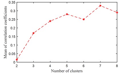
Fig. 6Decomposed modes of the mixed signal as shown in Fig. 3(a) using FMD and their ES results
Effectiveness of the proposed method is verified without considering the influence of noise through the analysis of the above simulation signals. White Gaussian noise is added to the original composite signal as shown in Fig. 3(a) with a signal noise ratio (SNR) of –5 dB, and the composite signal with noise is shown in Fig. 7(a), based on which the fault shock characteristics are basically submerged completely and difficult to be distinguished. Based on the method shown in Fig. 1, we still analyze the noised compound fault signal. In fact, some basis functions must be interfered by noise and converge to the random state, and some basis functions will converge to the form of fault features in the process of SISC feature self-learning. At this time, there must be morphological differences between the basis functions that converge to the random state, and the basis functions that converge to the fault feature, so these basis functions that converge to the random state can be considered as a component of the mixed signal. The above mentioned method and process are still applicable, but there is an additional random component. Fig. 7(b) shows the 8 basis functions after the SISC self-learning process, from which it could be observed that some basis functions exhibit fault shock characteristics, and some basis functions are disturbed by noise and converge to the random state. The mean value of the Person correlation coefficient is calculated for each number of clusters, and its relationship with the number of clusters is shown in Fig. 7(c), in which is smallest when the number of clusters is 3, so the optimal number of clusters is estimated to be 3, that is, the number of fault sources is 3. Similarly, the optimal number of fault sources is used to apply FMD on the original composite fault signal, and the final analysis results are given in Fig.8, based on which satisfactory fault features are extracted.
Fig. 7Verification using simulated signal with added noise
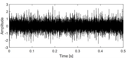
a) The mixed signal as shown in Fig. 3(a) | with added strong background noise
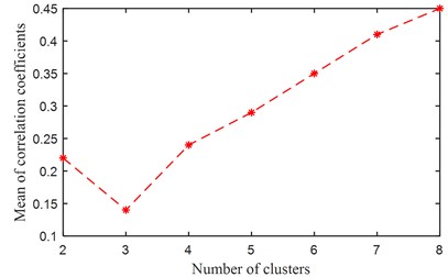
b) The mean value of correlation coefficients for each clustering number (Simulated signal with noise)
c) The learned basis functions of the signal as shown in Fig. 7(a)
5. Experiment
Three kinds of rolling bearing’ compound faults are analyzed in the section: 1) Outer ring fault and inner ring fault (OI). 2) Outer ring fault and ball fault (OB). 3) Outer ring fault and inner ring fault and ball fault (OIB). Fig. 9(a) is the test rig, and the test bearing is installed on the bearing seat at the outer end of the test bench, and its inner ring is assembled with the drive shaft, which is driven by the motor through the synchronous belt. Install acceleration sensors at the horizontal and vertical positions of the bearing housing (this experiment only needs the signal collected from one single channel). Fig. 9(b) is the signal acquisition system, which uses the NI PXI hardware platform and LabVIEW software development platform. In the experiment, the rotational speed of the main drive shaft is 800 r/min, and the sampling frequency of the signal acquisition system is 8192. The model of the test bearing is NU205, and the faults of its various components are processed by electrical discharge machining (EDM). The actual pictures of faults occurring on the outer ring, inner ring and rolling elements are shown in Fig. 10(a)-(c). Table 1 is the main geometric parameters of the test bearing, and Table 2 gives the theoretical fault characteristic frequency.
Fig. 8Decomposed modes of the mixed signal with noise as shown in Fig. 7(a) using FMD and their ES results
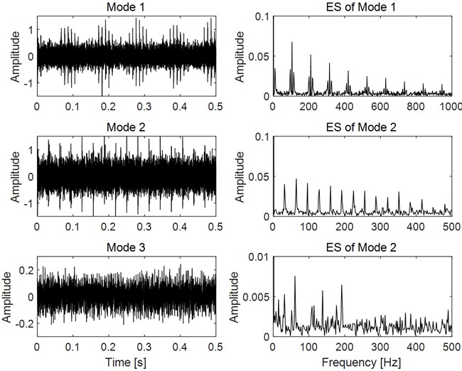
Fig. 9Experimental rig and the signal collection system
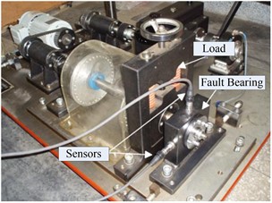
a) Test rig
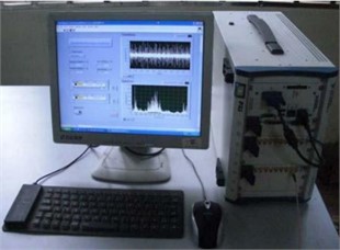
b) Signal collection system
Fig. 10Different fault of rolling element bearing created by EDM
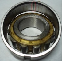
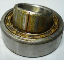
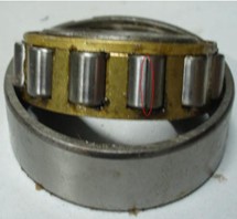
Table 1Geometrical parameters of bearing NU205
Type | Number of balls | Ball diameter (mm) | pitch diameter (mm) | Contact angle (°) |
NU205 | 12 | 7.5 | 39 | 0 |
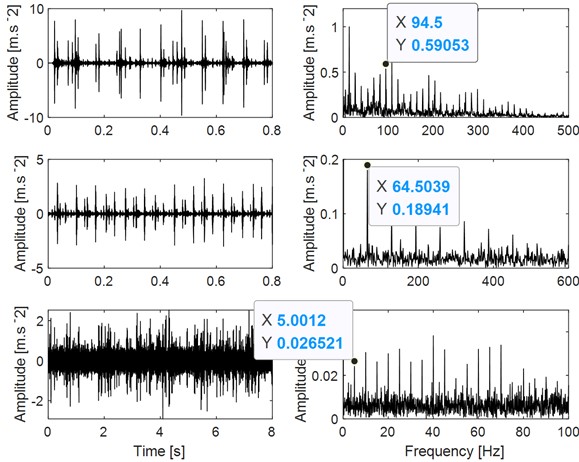
Fig. 11(a) and Fig. 11(b) show the time domain waveforms of three kinds of compound faults and their corresponding envelope spectrum analysis results respectively. Though some FCFs could be observed in Fig. 11(b), the features are not clear enough to verify the compound faults arising on different components of the test bearing: ES result of OI is complex, and the inner ring FCF 95 Hz and its harmonics, the outer ring FCF 65 Hz and its harmonics, and the rotating frequency components are all intertwined in the same envelope spectrum. In the ES of OB, only the outer ring FCF and its multiplier component can be seen, indicating that the energy of the outer ring fault excitation is very large, while the characteristic energy caused by the rolling defect is very small, and the ball fault cannot be detected effectively in the envelope spectrum. Various frequency components in the ES of OIB are complex, and various fault components have certain reactions. Unfortunately, all of the reactions are not obvious enough. Besides, the ideal results are to separate the original compound fault signal into several different single components.
Fig. 11Time domain waveforms of the rolling bearing’ three kinds of compound faults with their envelope spectrums
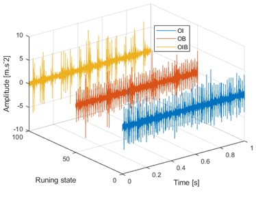
a) Time domain waveforms of the rolling bearing’ three kinds of compound faults
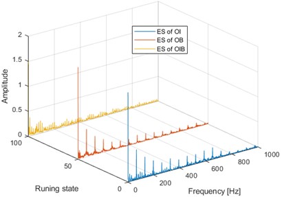
b) ES results of the signal as shown in Fig. 11(a)
Fig. 12The learned basis functions of the three kinds of signals as shown in Fig. 11(a)
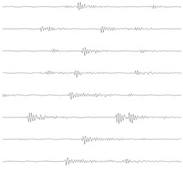
a) OI
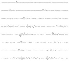
b) OB
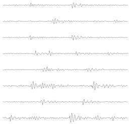
c) OIB
The proposed method is applied on the three kinds of signals in Fig. 11(a) respectively, and the parameters of the algorithm are the same as those in the simulation: the length of the signal segment is 1024, the overlap rate is 50 %, the length of basis function is 256, and the number of basis functions is 8. The eight self-learning time domain features are shown in Fig. 12, in which the number a~c corresponds to the three types of observation signals given in Fig. 11(a) respectively. The relationship between the average value of the Pearson correlation coefficient and the number of clusters of the three states are given in Fig. 13, based on which it can be seen that the first two observed signals both reach the minimum value when the cluster number is 2, and the third observed signal reaches the minimum value when the cluster number is 3. Based on the above analysis results, it is verified that the estimated source number in the experiment is consistent with the actual source number, so the above process also verifies the effectiveness of the fault source number estimation method.
Fig. 13The mean value of correlation coefficients for each clustering number (The three kinds of signals as shown in Fig. 11(a))
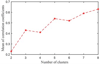
a) OI
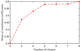
b) OB
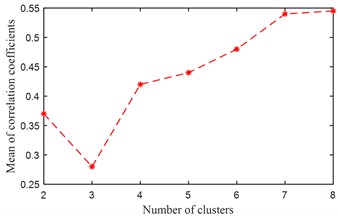
c) OIB
Fig. 14Decomposed modes of the compound fault signals as shown in Fig. 11(a) (OI, OB and OIB) using FMD and their ES results
a) OI
b) OB
c) OIB
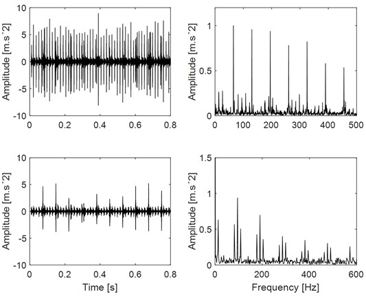
According to the fault sources number, the three compound fault signals given in Fig. 11(a) are processed by FMD, and the final result is given in Fig. 14: Fig. 14(a) is the decomposed modes of the compound fault signal (OI) and their ES results, based on which it could be observed that each mode represents the single fault component: the above mode represents the single component of outer ring fault and the bottom modes represents the single component of inner ring fault, and their corresponding ES results further verify the separation effectiveness. Similarly, the corresponding decomposed results of the OB and OIB compound fault signals are given in Fig. 14(b) and Fig. 14(c), based on which satisfactory separation results could be observed.
6. Comparison
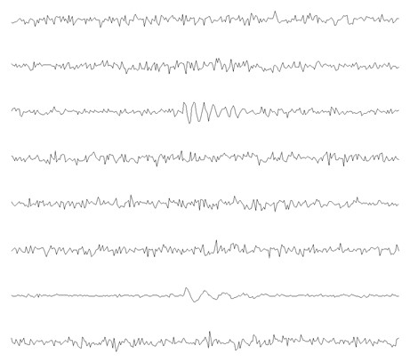
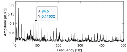
EEMD is the improvement of empirical mode decomposition (EMD), which not only retains the self-adaptability advantages of EMD, but also solves the problem of mode mixing. SCBSS could be realized by using EEMD to decompose the analyzed signal into several intrinsic mode function (IMFs), so EEMD is used for comparison firstly. Take the most complex compound fault signal in Fig. 11(a) as the object, that is OIB, and its corresponding EEMD analysis result is given in Fig. 15(a) (only 8 intrinsic mode function (IMFs) are presented).
Fig. 15Decomposed result of the signal as shown in Fig. 11(a) (OIB) using EEMD and the ES results of selected imfs
a) Decomposed result of the signal as shown in Fig. 11(a) (OIB) using EEMD
b) Envelope spectrum result of the imf1 as shown in Fig. 15(a)
c) Envelope spectrum result of the imf2 as shown in Fig. 15(a)
d) Envelope spectrum result of the imf3 as shown in Fig. 15(a)
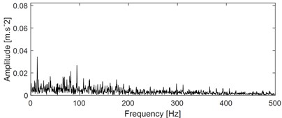
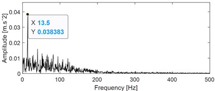
The calculated kurtosis values of the eight IMFs show that the first three IMFs (imf1-imf3) have the largest kurtosis value, which proves that they contain more shock fault characteristic components. Fig. 15(b), (c), and (d) are the ES analysis results of the three IMFs respectively. Based on the envelope spectrum results in Fig. 15(b), only the FCF of the inner ring can be extracted, while the FCFs of outer ring and rolling balls cannot be extracted effectively. The superiority of FMD for blind source separation of composite fault signals compared with EEMD is proved. In addition, EEMD still has the problem that it cannot judge the number of fault sources effectively during blind source separation. It is often necessary to judge the corresponding component manually according to the kurtosis index of each IMF, which has great chance to extract fault feature.
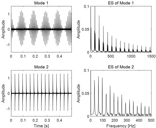
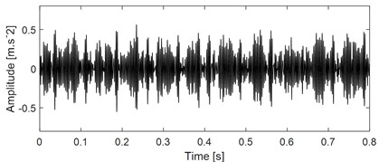
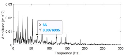
VMD could be used for SCBSS similar as EEMD theoretically, so it is also used here for comparison. Firstly, VMD is used to decompose the signal in Fig. 11(a) into several modes, and the decomposed result are presented in Fig. 16(a), (c) and (e). The number of decomposition mode is set as 3. Subsequently, apply ES analysis on the three modes and their corresponding results are shown in Fig. 16(b), (d) and (f). It could be observed that the outer ring and inner ring fault could be identified based on Fig. 16(b) and (d) respectively, the ball fault could not be identified based on Fig. 16(f). Besides, there are existing mode mixing between Mode 2 and Mode 3, because they both reflect inner ring fault. This comparison further verifies the superiority of the proposed method over VMD.
Fig. 16Decomposed result of the signal as shown in Fig. 11(a) (OIB) using VMD and the ES results of the obtained Modes
a) Mode 1
b) Envelope spectrum result of the imf1 as shown in Fig. 16(a)
c) Mode 2
d) Envelope spectrum result of the imf1 as shown in Fig. 16(c)
e) Mode 3
f) Envelope spectrum result of the imf1 as shown in Fig. 15(e)
7. Conclusions
As for the problem of SCBSS, one of the challenges is to determine the number of fault sources accurately. This paper presents a new method to solve the above difficulty by combining sparse decomposition self-learning dictionary with FMD. The sparse decomposition self-learning dictionary naming SISC is used for determining the optimal number of fault sources correctly, and the FMD method is used to separate the observed single channel fault signal into multiple single components using the determined fault sources number. Firstly, the feasibility is verified by applying the proposed method on the simulated compound fault signal of rolling bearing. Furthermore, the noise robustness of the proposed is also verified by simulation. Subsequently, the effectiveness of the proposed is verified by experimental signal. Finally, the advantage of the proposed over the other two TF methods (EEMD and VMD) is also presented by comparison study.
The current research of the paper mainly focuses on SCBSS of rolling bearing under stable operating speed. Compared with constant speed operating environment, the collected information reflecting the operating status of equipment under variable speed conditions is more challenging to diagnose due to speed fluctuations, and the diagnosis of compound faults in rolling bearing under variable speed condition is even more difficult. I believe that the proposed method combines the advantages of sparse representation self-learning dictionary algorithm (SISC) and FMD, and has great potential in the application of composite fault diagnosis of rolling bearings under variable speed conditions. In the future research, the proposed method will be combined with the order tracking analysis to expand its research on fault diagnosis of rotating machinery under variable speed condition. Besides, how to further expand from theory to more practical applications, I believe there is still a very long way to go. Of course, this is not denying theoretical research. Theoretical research can never stop, but the transformation of theoretical achievements requires the joint efforts of all scholars.
References
-
P. C. Jena, D. R. Parhi, and G. Pohit, “Dynamic investigation of FRP cracked beam using neural network technique,” Journal of Vibration Engineering and Technologies, Vol. 7, No. 6, pp. 647–661, Jul. 2019, https://doi.org/10.1007/s42417-019-00158-5
-
P. P. Sarada, P. C. Jena, and R. R. Dash, “Dynamic analysis of laminated composite beam using Timoshenko beam theory,” International Journal of Engineering and Advanced Technology, Vol. 8, No. 6, pp. 190–196, Aug. 2019.
-
S. P. Parida and P. C. Jena, “Selective layer-by-layer fillering and its effect on the dynamic response of laminated composite plates using higher-order theory,” Journal of Vibration and Control, Vol. 29, No. 11-12, pp. 2473–2488, Apr. 2022, https://doi.org/10.1177/10775463221081180
-
S. P. Parida, P. C. Jena, S. R. Das, D. Dhupal, and R. R. Dash, “Comparative stress analysis of different suitable biomaterials for artificial hip joint and femur bone using finite element simulation,” Advances in Materials and Processing Technologies, Vol. 8, No. sup3, pp. 1741–1756, Oct. 2022, https://doi.org/10.1080/2374068x.2021.1949541
-
Pankaj Charan, Dayal R. Parhi, and G. Pohit, “Theoretical, numerical (FEM) and experimental analysis of composite cracked beams of different boundary conditions using vibration mode shape curvatures,” International Journal of Engineering and Technology, Vol. 6, No. 2, pp. 509–518, May 2014.
-
P. C. Jena, “Identification of crack in SiC composite polymer beam using vibration signature,” Materials Today: Proceedings, Vol. 5, No. 9, pp. 19693–19702, Jan. 2018, https://doi.org/10.1016/j.matpr.2018.06.331
-
S. P. Parida and P. C. Jena, “Free and forced vibration analysis of flyash/graphene filled laminated composite plates using higher order shear deformation theory,” Proceedings of the Institution of Mechanical Engineers, Part C: Journal of Mechanical Engineering Science, Vol. 236, No. 9, pp. 4648–4659, Oct. 2021, https://doi.org/10.1177/09544062211053181
-
P. C. Jena, G. Pohit, and D. R. Parhi, “Fault measurement in composite structure by fuzzy-neuro hybrid technique from the natural frequency and fibre orientation,” Journal of Vibration Engineering and Technologies, Vol. 5, No. 2, pp. 123–136, Apr. 2017.
-
L. Sun, K. Xie, T. Gu, J. Chen, and Z. Yang, “Joint dictionary learning using a new optimization method for single-channel blind source separation,” Speech Communication, Vol. 106, pp. 85–94, Jan. 2019, https://doi.org/10.1016/j.specom.2018.11.008
-
M. R. Mohebbian, M. W. Alam, K. A. Wahid, and A. Dinh, “Single channel high noise level ECG deconvolution using optimized blind adaptive filtering and fixed-point convolution kernel compensation,” Biomedical Signal Processing and Control, Vol. 57, p. 101673, Mar. 2020, https://doi.org/10.1016/j.bspc.2019.101673
-
Y. Li, W.-T. Zhang, and S.-T. Lou, “Generative adversarial networks for single channel separation of convolutive mixed speech signals,” Neurocomputing, Vol. 438, pp. 63–71, May 2021, https://doi.org/10.1016/j.neucom.2021.01.052
-
Y. Hao, L. Song, M. Wang, L. Cui, and H. Wang, “Underdetermined source separation of bearing faults based on optimized intrinsic characteristic-scale decomposition and local non-negative matrix factorization,” IEEE Access, Vol. 7, pp. 11427–11435, Jan. 2019, https://doi.org/10.1109/access.2019.2892559
-
X. Zhao, Y. Qin, C. He, and L. Jia, “Underdetermined blind source extraction of early vehicle bearing faults based on EMD and kernelized correlation maximization,” Journal of Intelligent Manufacturing, Vol. 33, No. 1, pp. 185–201, Sep. 2020, https://doi.org/10.1007/s10845-020-01655-1
-
H. Sun, H. Wang, and J. Guo, “A single-channel blind source separation technique based on AMGMF and AFEEMD for the rotor system,” IEEE Access, Vol. 6, pp. 50882–50890, Jan. 2018, https://doi.org/10.1109/access.2018.2868643
-
G. Li, G. Tang, G. Luo, and H. Wang, “Underdetermined blind separation of bearing faults in hyperplane space with variational mode decomposition,” Mechanical Systems and Signal Processing, Vol. 120, pp. 83–97, Apr. 2019, https://doi.org/10.1016/j.ymssp.2018.10.016
-
K. Wang, Q. Hao, X. Zhang, Z. Tang, Y. Wang, and Y. Shen, “Blind source extraction of acoustic emission signals for rail cracks based on ensemble empirical mode decomposition and constrained independent component analysis,” Measurement, Vol. 157, p. 107653, Jun. 2020, https://doi.org/10.1016/j.measurement.2020.107653
-
Z. Li, Y. Jiang, Q. Guo, C. Hu, and Z. Peng, “Multi-dimensional variational mode decomposition for bearing-crack detection in wind turbines with large driving-speed variations,” Renewable Energy, Vol. 116, pp. 55–73, Feb. 2018, https://doi.org/10.1016/j.renene.2016.12.013
-
Z. Li, X. Yan, X. Wang, and Z. Peng, “Detection of gear cracks in a complex gearbox of wind turbines using supervised bounded component analysis of vibration signals collected from multi-channel sensors,” Journal of Sound and Vibration, Vol. 371, pp. 406–433, Jun. 2016, https://doi.org/10.1016/j.jsv.2016.02.021
-
J. Lu, W. Cheng, D. He, and Y. Zi, “A novel underdetermined blind source separation method with noise and unknown source number,” Journal of Sound and Vibration, Vol. 457, pp. 67–91, Sep. 2019, https://doi.org/10.1016/j.jsv.2019.05.037
-
Q. Ni, J. C. Ji, K. Feng, and B. Halkon, “A fault information-guided variational mode decomposition (FIVMD) method for rolling element bearings diagnosis,” Mechanical Systems and Signal Processing, Vol. 164, p. 108216, Feb. 2022, https://doi.org/10.1016/j.ymssp.2021.108216
-
G. Tang, G. Luo, W. Zhang, C. Yang, and H. Wang, “Underdetermined blind source separation with variational mode decomposition for compound roller bearing fault signals,” Sensors, Vol. 16, No. 6, p. 897, Jun. 2016, https://doi.org/10.3390/s16060897
-
Y. Miao, B. Zhang, C. Li, J. Lin, and D. Zhang, “Feature mode decomposition: new decomposition theory for rotating machinery fault diagnosis,” IEEE Transactions on Industrial Electronics, Vol. 70, No. 2, pp. 1949–1960, Feb. 2023, https://doi.org/10.1109/tie.2022.3156156
-
R. Duan and Y. Liao, “Impulsive feature extraction with improved singular spectrum decomposition and sparsity-closing morphological analysis,” Mechanical Systems and Signal Processing, Vol. 180, p. 109436, Nov. 2022, https://doi.org/10.1016/j.ymssp.2022.109436
-
J.-H. Lee, “Enhancement of decomposed spectral coherence using sparse nonnegative matrix factorization,” Mechanical Systems and Signal Processing, Vol. 157, p. 107747, Aug. 2021, https://doi.org/10.1016/j.ymssp.2021.107747
-
E. Eqlimi, B. Makkiabadi, N. Samadzadehaghdam, H. Khajehpour, F. Mohagheghian, and S. Sanei, “A novel underdetermined source recovery algorithm based on k-sparse component analysis,” Circuits, Systems, and Signal Processing, Vol. 38, No. 3, pp. 1264–1286, Aug. 2018, https://doi.org/10.1007/s00034-018-0910-9
-
G. Li, G. Tang, H. Wang, and Y. Wang, “Blind source separation of composite bearing vibration signals with low-rank and sparse decomposition,” Measurement, Vol. 145, pp. 323–334, Oct. 2019, https://doi.org/10.1016/j.measurement.2019.05.099
-
H. C. Wang, “Blind source extraction of rolling bearings’ multi-type faults based on self-learned sparse atomics,” Proceedings of the Institution of Mechanical Engineers, Part C: Journal of Mechanical Engineering Science, Vol. 233, No. 13, pp. 4531–4542, Feb. 2019, https://doi.org/10.1177/0954406219827163
About this article

The research is supported by the National Natural Science Foundation (approved grant: U1804141), the Key Science Technology Research Project of the Henan Province (approved grant: 232102221039).
The datasets generated during and/or analyzed during the current study are available from the corresponding author on reasonable request.
The authors declare that they have no conflict of interest.
