Abstract
The buckling behavior of tubular string is critical for safe oil and gas resource development. In practical engineering, the buckling of tubular string can appear in different development phases, such as casing putting into wellbore, BHA drilling rock, pipeline buckling, etc. Therefore, in this paper, the buckling behavior and buckling evolution of the tubular string are explored considering friction in horizontal wells. By applying the principles of static equilibrium and beam-string theory, an established theoretical model is utilized to examine the buckling behavior of tubular string. The critical load for sinusoidal buckling is determined by using both the series and trial function methods, and a comparison is made between the results obtained from these two techniques. In addition, perturbation analysis is used to obtain the angular displacement's configuration function in the helical buckling post-buckling state. To validate the model's effectiveness, a comprehensive analysis of the numerical results is performed, considering both sinusoidal and helical buckling scenarios. The research findings demonstrate that both the series method and the trial function method can effectively analyze sinusoidal buckling with high accuracy. The presence of friction significantly impedes the buckling behavior of the tubular string. Moreover, friction’s influence causes a gradual decline in the efficiency of transmitting axial forces along the wellbore axis.
Highlights
- The mechanical model of the microelement of pipe string in the horizontal well is established.
- The buckling equation of pipe string is solved using the series method and trial function method.
- The relationship of the transfer efficiency of the axial force on the friction force is revealed.
- The evolution of sinusoidal buckling to helical buckling is studied.
1. Introduction
Tubular string buckling is a well-known concern that often arises in drilling engineering, which leads to severe consequences, such as wellbore enlargement [1], wellbore collapse [2, 3], pipe-sticking, and equipment damage [4, 5]. Therefore, it is essential to understand the buckling behavior of tubular string as the tubular string buckling directly impacts drilling safety, drilling efficiency, and cost control [6-8]. A comprehensive understanding of buckling behavior is in favor of improving the extension of horizontal wells, optimizing drilling parameters, and reducing downhole complexity. The study of tubular string buckling poses notable challenges in petroleum drilling, which primarily arise from challenges in experimental observation, complex underground conditions, interactions between tubular string and wellbore, and realistic numerical simulations. In this case, the accurate model for simulating buckling behavior in the tubular string is less improved and perfected [9].
However, the problem of tubular string buckling widely exists in different development phases of oil and gas resources. In many workover treatments, coiled tubing (CT) is a crucial facility for carrying workover tools [10, 11]. Inaccessibility of CT is faced in the drilling completion phase, more than 30-40 % of long multilateral wells fail in CT entering into the wellbore due to severe interaction within CT and wall [12, 13]. Moreover, Casing plays a role in supporting and protecting the well wall, storing or producing oil, and controlling well pressure. Small-size casing string usually suffers from severe buckling or bending when put into the wellbore, which causes the strength failure of casing string or decreases passing ability.
In an earlier study, Lubinski systematically investigated the buckling behavior and characteristics of tubular pipe in straight wells and derived the formula for critical buckling load [14, 15]. Paslay and Bogy employed the energy method to investigate the stability of a circular rod in an inclined cylindrical cylinder, first [16]. Paslay and Dawson further concerned the buckling problem by using stability criteria [17], and it was found that the critical load of sinusoidal buckling was given in deviated wellbores, and the findings were confirmed by numerous scholars [18, 19]. Based on previous research, Mitchell observed that the tubular string appeared as a complex transitional section between sinusoidal and helical buckling [20]. There was a debate regarding the critical load of helical buckling as many scholars applied different methods and assumptions for solving analytical solutions [21-27]. McCann and Suryanarayana conducted laboratory-scale experiments in actual drilling operations and found that the experimental results significantly deviated from theoretical results as the existence of friction was neglected [28]. Gao Guohua and Msika’s buckling model considered the friction and derived the differential equation by employing the energy method [29, 30], it was found that the friction and axial force determine the buckling condition of the string together. To sum up, Lubinski's work provided an important theoretical basis for investigating tubular string buckling, however, the computation accuracy of theoretical buckling was rough as many parameters and conditions are ignored in the model. The energy method proposed by Paslay for studying tubular string buckling revealed the evolution process of buckling behavior in different axial loads and friction forces. Mitchell's work was crucial, but little provided concrete proof of the existence of the transitional section. Although the existence of friction factor on the critical load of tubular pipe buckling was concerned by Gao Guohua and Miska, the axial load was less affected by friction in the established model.
To reveal the evolution of buckling behavior and characteristics of tubular string in the presence of friction in horizontal wells, three important issues need to be addressed. Firstly, the tubular string, with complex geometric shapes and nonlinear mechanics properties, is usually in contact with the wellbore wall, which makes it difficult to make appropriate assumptions and establish theoretical models. Secondly, high nonlinearity and uncertain solutions are exhibited in the buckling differential equations of the tubular string, therefore, selecting suitable methods for solving these buckling equations is crucial when studying tubular string buckling. Lastly, the presence of friction makes the tubular string buckling more complex; compared to the case neglecting friction, the critical load of buckling is altered by the existence of friction; however, the explanation regarding alteration in critical load caused by friction in the tubular string is less provided nowadays. As a result, a more accurate and suitable modeling approach to capture the nonlinear contact is proposed in this paper. To find effective methods for handling the differential equation of buckling, the series method and trial function method is employed for exploring the sinusoidal buckling of tubular string, while the trial function method and perturbation method are given for studying helical buckling. Moreover, the complexity of the tubular string buckling due to friction is analyzed. Finally, the existence of the transitional section between sinusoidal and helical buckling has been confirmed.
2. Mechanical model of tubular string
The following assumptions are taken into account:
1) The wellbore is regarded as the inner wall of a straight cylinder lying horizontally.
2) The contact status is considered as continuous contact status.
3) The slender beam theory is applicable.
4) The deformation is within the elastic deformation range.
5) The tubular string slides in the cylindrical wellbore maintaining constant direction of motion.
6) Ignore torque and dynamic effects in the model.
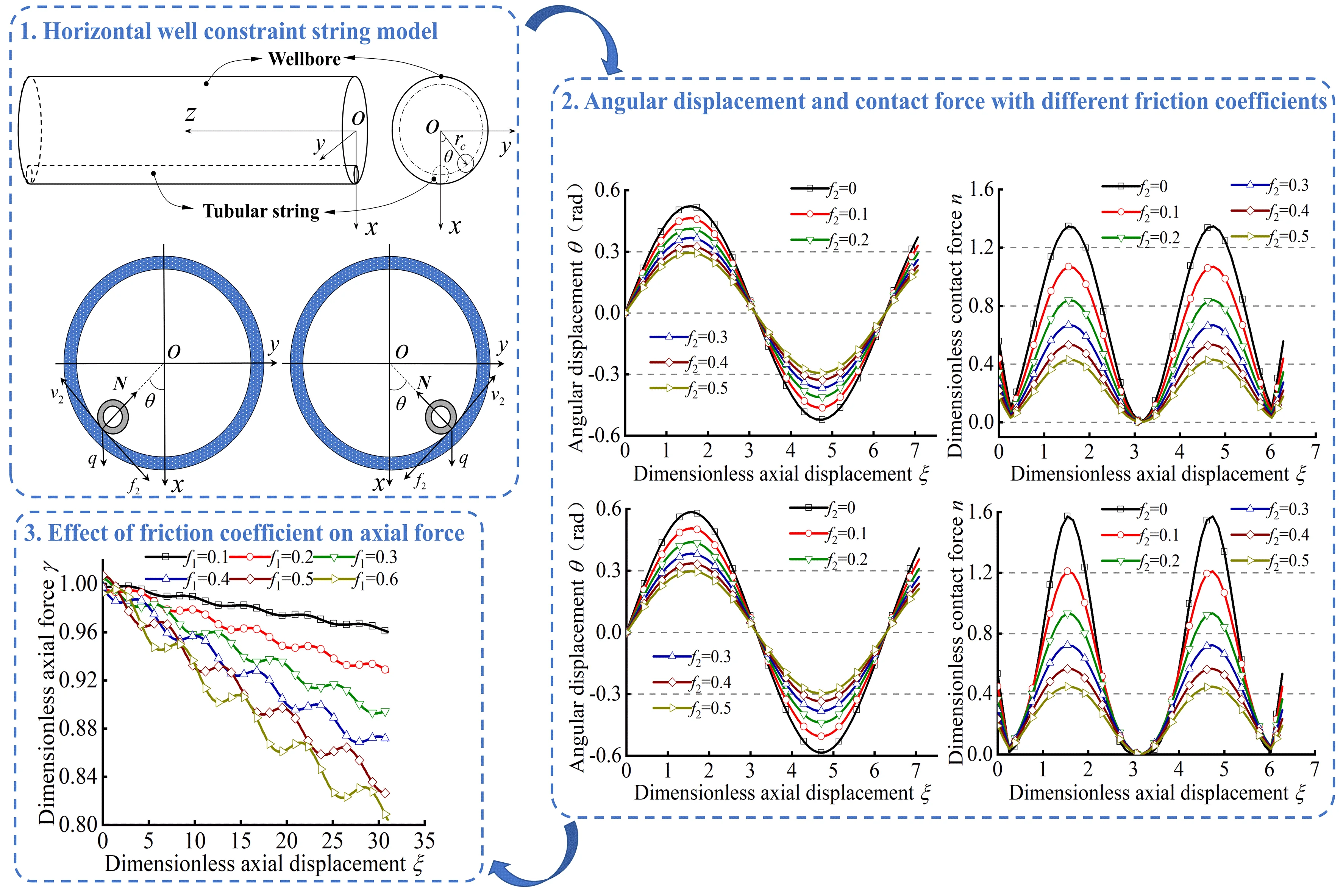
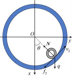
Fig. 1 depicts the tubular string being confined by the wellbore. It also shows the established Cartesian coordinate system -. The -axis goes straight down in line with gravity. The -axis is the same as the horizontal direction. The -axis direction is consistent with the direction of the wellbore centerline. The buckling differential equations can be derived using the principle of static equilibrium combined with geometric relations. Geometric relations in the established Cartesian coordinate system are given as follows:
where, is the vector diameter for any point on the tubular string, and (m) is the radial clearance between tubular string and wellbore. (rad) is the lateral angular displacement of tubular string at different positions. , , and represent unit direction vectors in the , , and axis in Cartesian coordinates, respectively.
Fig. 1Coordinate establishment of tubular string in horizontal well
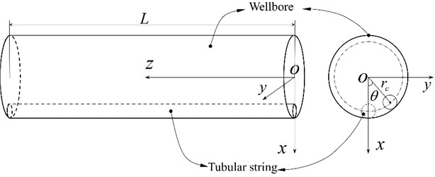
Fig. 2Mechanical model of the infinitesimal element of tubular string
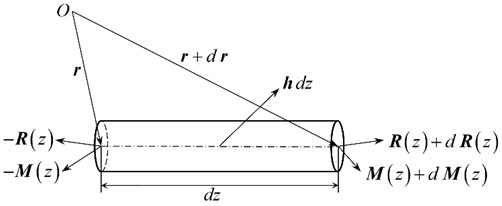
Fig. 2 illustrates the mechanical model of selected infinitesimal element. The micro-element segment is intercepted from the tubular string at . The external force acting on micro-element segment is . The per-unit length external force acting on the tubular string is denoted as . At position , the vector diameter is represented as , while the internal force and internal moment are denoted as and , respectively. At position , the vector diameter is expressed as , while the internal force and internal moment are given by and , respectively. The per-unit length moment of momentum of the tubular string is denoted as , and the material density of tubular string is given as . The tubular string’s cross-sectional area is represented by the symbol . Ignoring vibration damping in tubular string system and applying the momentum theorem and moment of momentum theorem can be obtained:
Ignoring the dynamic effect of tubular string, Eqs. (2) and (3) can be simplified as follows:
The deformation of tubular string buckling still belongs to small elastic deformation. Therefore, the relationship between moment and deflection related to the cross-section of the slender beam should be satisfied:
where, is the bending stiffness of tubular string.
The bending moment of cross-section can be further obtained as follows:
Fig. 3Different buckling conditions
a) initial linear state
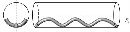
b) sinusoidal buckling state
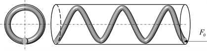
c) helical buckling state
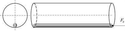
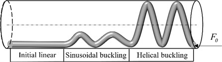
Buckling deformation of tubular string appears as axial force is gradually increased. Fig. 3 shows different deformations of the tubular string buckling at various axial forces. The tubular string is initially maintained in a linear shape, as illustrated in Fig. 3(a). The tubular string transitions from a linear shape to two-dimensional lateral buckling when remains below the critical load for sinusoidal buckling. Fig. 3(b) showcases the appearance of the sinusoidal buckling shape (three-dimensional buckling) in the tubular string when reaches the critical load for sinusoidal buckling. Finally, as is continually improved, the tubular string evolves into the helical buckling shape from the sinusoidal buckling shape, as depicted in Fig. 3(c). Therefore, the tubular string buckling is closely related to in the loading end of tubular string. As the friction is considered, the axial force transfer at the end of tubular string is changed, which finally affects the specific buckling process. The actual deformation of the whole tubular string is a combination of buckling states when applied in tubular string is large enough, as shown in Fig. 4.
Fig. 4Actual buckling combination of the tubular string
Guohua Gao and Mitchell described the friction direction in a cross section of tubular string in the drilling process. At the same time, the relationship of axial velocity and lateral velocity of tubular string in a certain cross section is also studied. Axial friction coefficient and lateral friction coefficient are presented by the relationship between and , respectively [29-32]:
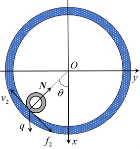
The tubular string maintains its initial straight shape when is below the critical load for sinusoidal buckling. However, the tubular string laterally slides when is equal to or more than the critical load, which certainly shortens the tubular string in the axial direction, therefore, the is the important factor affecting the initial buckling condition. Fig. 5 illustrates the contact condition of the tubular string and wellbore in the cross section.
Fig. 5Geometric model in cross-section of tubular string and wellbore
a)
b)
If the tubular string is laterally shifted to the right of center (Fig. 5(b), ), the force balance equation can be obtained as follows:
where, (N) represents the external force acting on the string when the tubular string is shifted to the right side of center ; (N) represents the contact force. The weight per unit length of the tubular string is denoted by (N/m).
When the tubular string is shifted to the left of center (Fig. 5 (a), 0), the same analysis method can be employed. Thus, we have:
where, (N) represents the external force acting on the tubular string when the tubular string is shifted to the left side of center .
Eq. (12) and Eq. (13) above can be synthesized into the following equation:
where, (N) represents the external force acting on the cross section of tubular string, and is used to determine the choice of plus or minus sign.
Combining Eqs. (1), (4), (5), (7), (8) and (14), we have:
where, (N) is the axial force at the loading end of tubular string.
There are three unknown parameters in the equations above, i.e., and . The dimensionless parameters and are introduced into Eqs. (15) to (17) [33-35]. Thus, Eqs. (15) to (17) can be converted into the following dimensionless expressions:
where, is the dimensionless parameter. Eqs. (18) to (20) are the buckling differential equations when the tubular string is affected by friction force (). It can be seen that the differential equations are coupled by angular displacement, contact force, and axial force.
3. Sinusoidal buckling analysis
3.1. Solution by the series method
The tubular string changes to two-dimensional lateral buckling from a linear shape as the axial force gradually increases. Then the sinusoidal buckling occurs, and the tubular string is deformed into a sinusoidal serpentine structure. According to the findings of Tianxiang Su [36], the configuration function of angular displacement of sinusoidal buckling of tubular string can be assumed as follows:
Because the sign function is nonlinear, is mainly determined by parameter , and the following formula can be obtained:
For simplifying the derivation process, considering that there is a dominant deformation configuration in sinusoidal buckling. Without losing generality, the configuration function of angular displacement can be directly expressed as the following formula:
Here, half-wave periods are assumed in sinusoidal buckling shape of tubular string, so the dimensionless length in this range can be given as . Then Fourier series coefficient can be simplified in the following formula:
Considering the relationship between velocity and friction, lateral sliding velocity mainly exists in the initial sinusoidal buckling condition. Assuming that axial velocity of tubular string is zero, therefore, we have and . Then, Eq. (18) can be calculated by the Galerkin method as follows:
By bringing Eq. (24) into the definite integral (26), the following formula can be obtained:
If friction is neglected, Eq. (27) becomes:
Therefore, the solution of can be obtained as:
It is important to mention that the tubular string undergoes a process from linear shape to curve shape in the beginning of sinusoidal buckling deformation. Therefore, the critical requirement for the initial condition of sinusoidal buckling is that the amplitude value () should be zero. Substituting this critical condition into Eq. (29) and converting it into engineering units, the following formula can be obtained:
Eq. (30) is the critical load for sinusoidal buckling of tubular string. Parameter should be satisfied by , and it can be concluded when the tubular string begins buckling deformation. Then, it can be obtained as follows by bringing this result into Eq. (30):
Referencing the previous study, Eq. (31) is agreement with the critical load of sinusoidal buckling of tubular string without considering friction in horizontal wells. However, it is evident from Eq. (27) that there is no zero solution for , which indicates the impossibility of tubular string being directly transited from linear shape to the sinusoidal buckling shape. This conclusion is well agreement with the conclusion obtained by Mitchell [32] and Su et al [36]. The deformation process is not only affected by friction but also disturbed by initial perturbation momentum. As the tubular string is in sinusoidal buckling, the critical axial force cannot be directly obtained from Eq. (27), which determines the maximum axial force for maintaining sinusoidal buckling. In addition, when , the minimum contact force can be obtained. Eq. (24) is directly substituted into Eq. (19), and the minimum contact force can be written as formula (32):
The condition that the tubular string maintains sinusoidal buckling equilibrium in the horizontal well is . So, Eq. (24) can be substituted into Eq. (19), and considering , the critical condition is obtained:
According to the reference Gao and Miska [29], it was concluded that the period of buckling shape of tubular string remains unchanged when the tubular string enters into the post-buckling state. However, when the axial force in the loading end of tubular string is gradually improved, the angular displacement amplitude is also gradually increased. Therefore, the relation between and can be simplified by assuming. The maximum axial force maintaining sinusoidal buckling shape can be gained by solving Eq. (34), and the helical buckling shape appears if the axial force of tubular string is further increased:
3.2. Solution by the trial function method
Similarly, and are found in the initial condition of sinusoidal buckling. The sign function of Eq. (18) is equal to 1 according to Deli Gao's conclusion. Therefore, Eqs. (18) and (19) can be rewritten as:
Eq. (35) and Eq. (36) are decoupled by introducing Eq. (36) into Eq. (35). Thus, the differential equation of tubular string buckling considering friction can be obtained as follows:
When tubular string occurs sinusoidal buckling, the configuration solution of angular displacement of tubular string is:
where, and are undetermined coefficients. Galerkin method is applied in Eq. (37), and we can obtain:
Eq. (40) can be determined by substituting Eq. (38) into Eq. (39), thus:
It can be seen that Eq. (40) is nonlinear. The contact force can obtain by introducing Eq. (38) into Eq. (36), and the expression of the minimum contact force can gain as follows:
Condition should be satisfied when the tubular string occurs sinusoidal buckling, and the maximum critical load for maintaining sinusoidal buckling can be calculated according to Eq. (40) under a specific frictional coefficient.
4. Helical buckling analysis
4.1. Analysis of the helical buckling by the trial function method
Eqs. (35) and (36) also are buckling differential equations of tubular string, which can be solved by the Galerkin method. But effect of gravity on the tubular string is neglected in the conventional approach for analyzing helical buckling. To enhance analysis accuracy and simplify the analytical buckling, a small perturbation can be added to tubular string based on prior research findings. When tubular string occurs helical buckling, the configuration solution of angular displacement of tubular string is:
When the axial force is more than the critical load of helical buckling, transverse sliding of tubular string is mainly occurred, and lateral friction ( and ) is restricted in the initial condition of helical buckling. Therefore, the same buckling differential equation as Eq. (35) and Eq. (36). Galerkin’s weighted residual method is employed in Eq. (35), we have:
By introducing Eq. (42) into Eq. (43), the nonlinear equation can be obtained, which determining the initial condition of the helical buckling of tubular string, i.e.:
When tubular string occurs helical buckling in horizontal wells, it means that the tubular string becomes a helical shape and contacts with wellbore wall. Therefore, the contact force must be satisfied by when angular displacement is locked in (the position at the top of the horizontal well). By introducing Eq. (42) into Eq. (36), the minimum contact force formula can be written as follows:
Eq. (45) can be considered as zero when the critical point . Combined with Eq. (44), numerical solutions of and under specific friction coefficient can be obtained.
4.2. Analysis of helical post-buckling by perturbation method
The helical post-buckling state is mainly affected by , while the initial helical buckling condition is mainly affected by the . Therefore, in the helical post-buckling state (, and ), buckling differential Eqs. (35) and (36) are rewritten into the following equations:
It is worth noting that is a tiny quantity (and notice that ), the two nonlinear equations can be solved by the perturbation method according to nonlinear Eqs. (46) and (47). At the same time, the angular displacement, contact force, and axial force are mutually coupled, which can be seen from the two nonlinear equations. Then the asymptotic solutions of angular displacement and axial force can be assumed as follows:
where and , in which is the unknown function.
In order to obtain the coefficients of each order of , substituting Eqs. (48) and (49) into Eqs. (46) and (47), the expression of zero-order of can be obtained as:
Eq. (50) is consistent with Mitchell, then can be solved as:
The expression of the first-order coefficient of is:
Let the right part of the equal sign of Eq. (52) be zero can get as follows:
By substituting this result into Eq. (51) can gain that:
Similarly, Eqs. (53) and (54) are introduced into Eq. (52), we have:
The solution of Eq. (55) is:
Similarly, the second-order can be obtained. Introducing Eqs. (48) and Eq. (49) into Eq. (20) can obtain:
Assuming and integrating Eq. (57), the following results can be obtained:
Based on Eq. (58), the axial force affected by axial friction in helical post-buckling state can be written as follows:
Bringing Eq. (59) into second-order , we can obtain:
It can be gained by solving Eq. (60):
Based on the results above, the approximate angular displacement of the helical post-buckling state affected by friction force can be given as follows:
By the perturbation method, Eq. (62) is the configuration solution of angular displacement of helical post-buckling considering axial friction, and the contact force can be obtained by introducing Eq. (62) into Eq. (47).
5. Numerical analysis and discussion
When the series method is employed to handle sinusoidal buckling, parameters and in Eq. (24) are affected by the friction coefficient , in this case, the function configuration of the angular displacement are sensitive to and . Consequently, it is important to investigate the relationship among parameters , and friction coefficient . When friction coefficient is in the range of 0-0.7, the numerical solution of parameters and in Eq. (34) can be obtained when . As shown in Fig. 6, the negative correlation is appeared between parameter and friction coefficient , which indicates that increasing friction coefficient leads to the decrease of angular displacement amplitude . Furthermore, the negative correlation is existed between parameter and friction coefficient . According to , it can be seen that the enhancement of friction force results in increase of axial force at the loading end of tubular string.
Fig. 6The change of Am and Q0with different f2
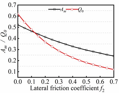
Fig. 7The series method in sinusoidal buckling
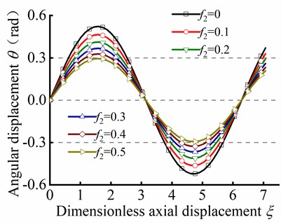
a) Curve of against
b) Curve of against
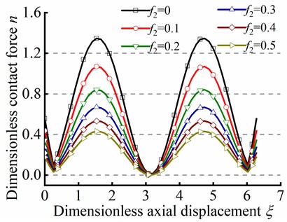
By the series method, the variations of angular displacement and dimensionless contact force are illustrated in Fig. 7(a) and Fig. 7(b), respectively. As depicted in Fig. 7(a), is decreased with the increase of friction coefficient , indicating that improving friction force leads to the increase of of tubular string. As depicted in Fig. 7(b), the peak of is decreased with the increase of friction coefficient , which implies that enhancing friction force results in the increase of peak value of . Furthermore, the minimum value of is larger than zero, which is agreement with the fact that the contact force is always greater than or equal to zero in the practical engineering.
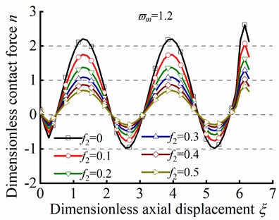
Fig. 8 illustrates the effect of the parameter ( and ) on sinusoidal buckling shape of tubular string. As can be seen from Eq. (24), the angular displacement period is negatively correlated with . When , the increase in friction coefficient is gone against the increase of contact force peak, but the minimum value of always be greater than zero, as shown in Figs. 8(a)-(c). On the contrary. When , the increase of is gone against the increase of the maximum value of , but the existence of a negative minimum value of is inconsistent with practical situations, as shown in Figs. 8(d)-(f). Therefore, is unreasonable in the practical engineering.
Fig. 8n in different ϖm by the series method in sinusoidal buckling
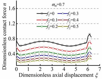
a)
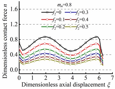
b)
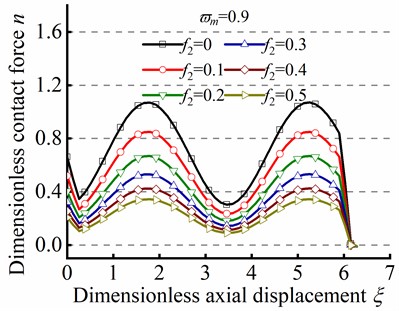
c)
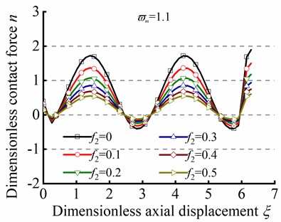
d)

e)
f)
It is necessary to investigate the relationship among parameters , , and friction coefficient when analyzing the sinusoidal buckling by using the trial function method. As shown in Eq. (38), the parameters , , and are also affected by the friction coefficient . Thus, combined with case of in Eq. (41), the numerical solution of , , and can be determined by Eq. (40) as 0-0.7. As displayed in Fig. 9, the negative correlation is exhibited between parameter and , however, the positive correlation is displayed between parameter and . Moreover, shows a negative correlation related to . Parameter reflects the amplitude of , parameter reflects the amplitude of the small perturbation of the angular displacement, and parameter represents the dimensionless axial force. The results show that with the increase of friction, is gradually decreased, is gradually increased, and is gradually decreased.
The variations of angular displacement and dimensionless contact force respected to dimensionless axial displacement can be caclucated by the trial function method, as depicted in Fig. 10(a) and Fig.10(b), respectively. Consistent with the conclusions drawn by the series method, the peak values of and is decreased by increasing friction coefficient and maintaining constant at the loading end. Moreover, the minimum value of is always greater than zero, which is well agreement with actual situation where the contact force is nonnegative.
Fig. 9The change of parameters a, b and Q0 in different f2
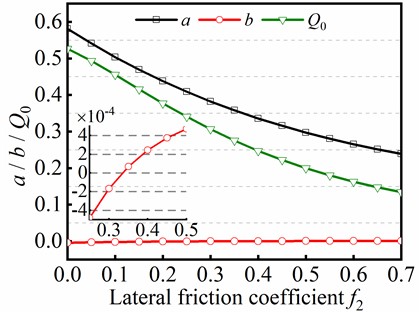
Fig. 10Trial function method in sinusoidal buckling
a) Curve of against
b) Curve of against
In this study, the sinusoidal buckling of tubular string was handled by employing the series method and the trial function method, respectively. The two methods firstly described the configuration function of sinusoidal buckling angular displacement , and then numerical solutions of specific parameters for solving the equations with different forms of configuration functions . The differences in the results of the two methods were compared based on (Dimensionless maximum axial force, which maintains sinusoidal buckling) and (Dimensionless axial load) introduced. Fig. 11 shows the curves of and changing with the lateral friction coefficient . Fig. 11(a) shows the variation of against obtained by the two methods, indicating that the increment of friction will increase the maximum critical load of sinusoidal buckling. Fig. 11(b) shows the variation of obtained by the two methods, indicating that the increment of friction will decrease the dimensionless axial force. The results obtained by the two methods have consistency. The maximum error of the maximum critical load of sinusoidal buckling is only 5.37 % at 0.7. The maximum error of the dimensionless axial force is 16.1 % at . However, the error is less than or equal to 4.18 % when , which indicates that the error of the two methods is small when friction force is considered in the mechanical model. Therefore, it can be concluded that the two methods can be employed to handle the sinusoidal buckling of tubular string.
Fig. 11Comparison of series method between trial function method
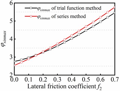
a) Curve of against
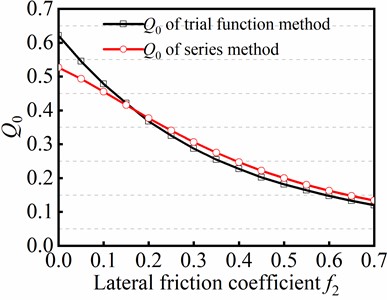
b) Curve of against
5.1. Numerical analysis of the helical buckling
Before analyzing helical buckling shape of tubular string, it is of great significance to discuss the transitional section between sinusoidal buckling and helical buckling. On account of the complexity and irregularity of the transitional section, it is difficult to provide a specific and accurate description for the transitional section in previous studies. In this study, the transitional section is analyzed by comparing (dimensionless maximum critical axial force, which maintains sinusoidal buckling) with (dimensionless critical axial force of helical buckling). The variations of and in different friction coefficient are shown in Fig. 12, the values of parameters and is risen with increasing the friction coefficient , which indicates that the varation of critical load is dtermined by friction coefficient .
Fig. 12Parameters ϕsinmax and ϕhel against f2
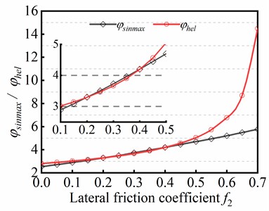
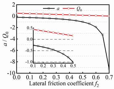
Fig. 13Parameters a and Q0 with respect to f2
When the friction coefficient , the difference between and is very small, indicating that the transitional section between sinusoidal buckling and helical buckling is weakly appeared in this case. However, when the friction coefficient , the difference between and is obviously found. Although friction coefficient more than 0.5 is rare in actual drilling engineering, the analysis results imply the existence of transitional section in buckling behavior of tubular string.
The trial function method is employed for analyzing helical buckling of tubular string in initial state, and the connection among parameters , and friction coefficient is discussed with numerical computation. Combining Eq. (44) with Eq. (45), the numerical solutions of parameters and can be obtained when . Fig. 13 shows the variation of parameters and with respected to friction coefficient , and it can be seen that parameters and areboth decreased as friction coefficient is risen. It shows that the amplitude fluctuation of angular displacement is affected by parameters and , and the greater the friction force, the greater the amplitude fluctuation.
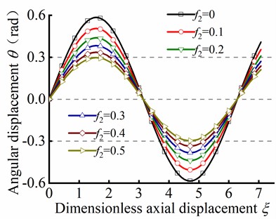
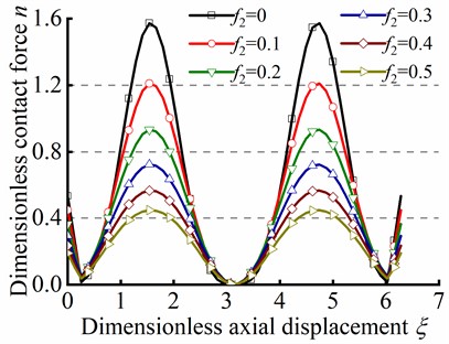
By substituting Eq. (42) into Eq. (35) and Eq. (36), the variation of and with respect to dimensionless axial displacement can be determined when the tubular string occurs helical buckling, as depicted in Fig. 14. It can be observed that when neglecting the friction coefficient, the angular displacement is approximately a straight line in Fig. 14(a). As the friction coefficient is increased, the angular displacement is weakly fluctuated as , and the fluctuation amplitude is risen with increasing friction coefficient . Moreover, there is an intersection point in the curve of the angular displacement in different friction coefficient. Before reaching the intersection point, exhibits a decreasing tendency as increases. Conversely, after the intersection point, the opposite phenomenon occurs, whereby the angular displacement increases as the friction coefficient increases. As depicted in Fig. 14(b), is decreased with increasing friction coefficient, which is indicated that decreases with increasing friction force.
Fig. 14The helical buckling of tubular string
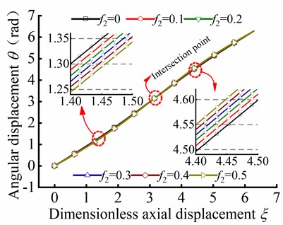
a) Curve of against
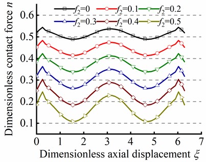
b) Curve of against
Finally, the post-buckling state of helical buckling of tubular string is concerned. In this condition, the distance of ends of tubular string is shorten as post-buckling state of helical buckling is appeared, therefore, the impact of the axial friction coefficient on post-buckling state is primarily discussed. The buckling differential equation of the tubular string in this situation is given by Eqs. (46) and (47). The mode function Eq. (62) and axial force Eq. (59) is obtained by using the perturbation method.
The value of the initial parameters for solving post-buckling mechanical behavior are listed in Table 1. Substituting Eq. (62) into Eq. (46), the numerical solution of the angular displacement can be obtained as axial friction coefficient is in range of 0.1-0.6. Fig. 15(b) shows the angular displacement of point A near the loading end of tubular string, and Fig. 15(c) shows the angular displacement of point B away from the loading end. It can be concluded that the angular displacement is decreased with the axial friction coefficient increase, and this indicates that angular displacement is decreased in different axial friction during the post-buckling state.
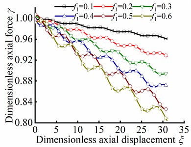
The relationship between and are obtained by substituting initial values and numerical results of , into Eq. (59). Fig. 16 shows the variation of dimensionless axial force with respected to dimensionless axial displacement . Based on the dimensionless axial force Eq. (20) and the introduced parameter, is represented the transfer efficiency of axial force along the axis direction in wellbore. It can be concluded from Fig. 16 that the transmission efficiency of axial force is decreased with the increase of the axial friction coefficient , which indicates that the axial force in the loading end is gradually decreased with the increase of displacement along the wellbore axis. The change of axial force is directly determined the critical load under different buckling conditions. Therefore, compared with the case neglecting friction, the existence of friction causes the change of critical load in different buckling conditions, which is the main reason of the evolution among different buckling conditions. The higher the friction coefficient is, the lower the axial force transfer efficiency is; and the higher the critical load in different buckling conditions is. As a result, higher axial force is exerted at the loading end to make the tubular string reach the critical load in corresponding buckling conditions.
Fig. 15Parameter θ in different ξ and f1 in helical post-buckling
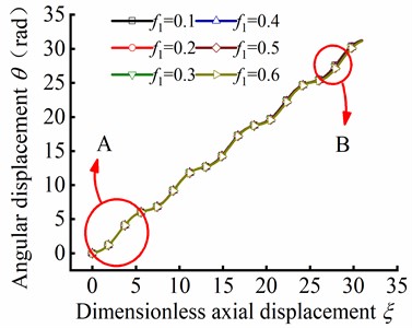
a) Curve of against
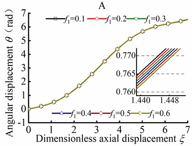
b) Local amplification A
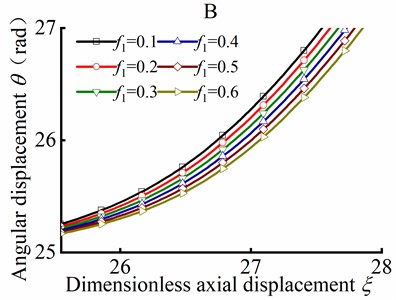
c) Local amplification B
Table 1The numerical value of the initial parameter
Parameter | Numerical value |
Wellbore diameter, (m) | 0.1651 |
Wellbore length, (m) | 100 |
Outside diameter of the tubular string, (m) | 0.1016 |
Inside diameter of the tubular string, (m) | 0.0823 |
Young’s modulus, (Pa) | 2.1×10¹¹ |
Weight per unit length of the tubular string, (kg/m) | 19.26 |
Axial force at the loading end, (N) | 120000 |
Coefficient of friction, | 0.1~0.6 |
Fig. 16Parameter γ in different ξ and f1 in helical post-buckling
6. Conclusions
The following significant conclusions are acquired:
1) During the sinusoidal buckling state, is decreased with the increase of friction coefficient , indicating that improving friction force leads to the increase of angular displacement of tubular string. The peak of is decreased with the increase of friction coefficient , which implies that enhancing friction force results in the increase of peak value of . Furthermore, the lowest value of is larger than zero, which is agreement with the fact that is always greater than or equal to zero in practical engineering.
2) In the helical buckling shape, the values of (dimensionless maximum critical axial force maintaining sinusoidal buckling) and (dimensionless critical axial force of helical buckling) are risen with increasing the friction coefficient , which indicates that the varation of critical load is determined by friction coefficient . When the friction coefficient , the difference between and is very small, it is demonstrated that the transitional section between sinusoidal buckling and helical buckling is weakly appeared in this case. However, when the friction coefficient , the difference between and is obviously found. Although friction coefficient more than 0.5 is rare in actual drilling engineering, the analysis results implies the existence of transitional section in buckling behavior of tubular string.
3) When the tubular string occurs helical post-buckling, the distance between ends of tubular string shortens as the severe spiral shape appears due to larger axial force at the end of tubular string, therefore, the impact of the axial friction coefficient on helical post-buckling state is primarily discussed. It can be concluded that the angular displacement decreases with an increase in the axial friction coefficient . This indicates that the angular displacement is reduced under axial friction during the helical post-buckling state.
4) The change of axial force is directly determined the critical load under different buckling conditions. Therefore, compared with the case neglecting friction, the existence of friction causes the change of critical load in different buckling conditions, which is the main reason of the evolution among different buckling conditions. The higher the friction coefficient is, the lower the axial force transfer efficiency is; and the higher the critical load in different buckling conditions is. As a result, higher axial force is exerted at the loading end to make the tubular string reach the critical load in corresponding buckling conditions.
References
-
Q. Li, L. Liu, B. Yu, L. Guo, S. Shi, and L. Miao, “Borehole enlargement rate as a measure of borehole instability in hydrate reservoir and its relationship with drilling mud density,” Journal of Petroleum Exploration and Production Technology, Vol. 11, No. 3, pp. 1185–1198, Feb. 2021, https://doi.org/10.1007/s13202-021-01097-2
-
W. Zhang, J. Gao, K. Lan, X. Liu, G. Feng, and Q. Ma, “Analysis of borehole collapse and fracture initiation positions and drilling trajectory optimization,” Journal of Petroleum Science and Engineering, Vol. 129, pp. 29–39, May 2015, https://doi.org/10.1016/j.petrol.2014.08.021
-
Z. Liu, M. Chen, Y. Jin, X. Yang, Y. Lu, and Q. Xiong, “Calculation model for borehole collapse volume in horizontal openhole in formation with multiple weak planes,” Petroleum Exploration and Development, Vol. 41, No. 1, pp. 113–119, Feb. 2014, https://doi.org/10.1016/s1876-3804(14)60013-6
-
D. Song et al., “Drilling performance analysis of impregnated micro bit,” Mechanical Sciences, Vol. 13, No. 2, pp. 867–875, Oct. 2022, https://doi.org/10.5194/ms-13-867-2022
-
D. Song, Z. Ren, Y. Yang, and H. Ren, “Research on cutter surface shapes and rock breaking efficiency under high well temperature,” Geoenergy Science and Engineering, Vol. 222, p. 211422, Mar. 2023, https://doi.org/10.1016/j.geoen.2023.211422
-
P. Amir-Heidari, R. Maknoon, B. Taheri, and M. Bazyari, “Identification of strategies to reduce accidents and losses in drilling industry by comprehensive HSE risk assessment-A case study in Iranian drilling industry,” Journal of Loss Prevention in the Process Industries, Vol. 44, pp. 405–413, Nov. 2016, https://doi.org/10.1016/j.jlp.2016.09.015
-
M. T. Albdiry and M. F. Almensory, “Failure analysis of drillstring in petroleum industry: A review,” Engineering Failure Analysis, Vol. 65, pp. 74–85, Jul. 2016, https://doi.org/10.1016/j.engfailanal.2016.03.014
-
K. A. Macdonald and J. V. Bjune, “Failure analysis of drillstrings,” Engineering Failure Analysis, Vol. 14, No. 8, pp. 1641–1666, Dec. 2007, https://doi.org/10.1016/j.engfailanal.2006.11.073
-
Z. Li, C. Zhang, and G. Song, “Research advances and debates on tubular mechanics in oil and gas wells,” Journal of Petroleum Science and Engineering, Vol. 151, pp. 194–212, Mar. 2017, https://doi.org/10.1016/j.petrol.2016.10.025
-
“An Introduction to Coiled Tubing: History, Applications, and Benefits,” International Coiled Tubing Association, 2005.
-
Y. S. Yang, “Understanding factors affecting coiled-tubing engineering limits,” in Society of Petroleum Engineers, 1999.
-
J. Yeung, J. Li, J. Lee, and X. Guo, “Evaluation of lubricants performance for coiled tubing application in extended reach well,” in SPE/ICoTA Coiled Tubing and Well Intervention Conference and Exhibition, Mar. 2017, https://doi.org/10.2118/184810-ms
-
S. Livescu, S. Craig, and T. Watkins, “Challenging the industry’s understanding of the mechanical friction reduction for coiled tubing operations,” in SPE Annual Technical Conference and Exhibition, Oct. 2014, https://doi.org/10.2118/170635-ms
-
A. Lubinski, “A study of the buckling of rotary drilling strings,” Drilling and Production Practice, 1950.
-
A. Lubinski and W. S. Althouse, “Helical buckling of tubing sealed in packers,” Journal of Petroleum Technology, Vol. 14, No. 6, pp. 655–670, Jun. 1962, https://doi.org/10.2118/178-pa
-
P. R. Paslay and D. B. Bogy, “The stability of a circular rod laterally constrained to be in contact with an inclined circular cylinder,” Journal of Applied Mechanics, Vol. 31, No. 4, pp. 605–610, Dec. 1964, https://doi.org/10.1115/1.3629721
-
R. Dawson, “Drill pipe buckling in inclined holes,” Journal of Petroleum Technology, Vol. 36, No. 10, pp. 1734–1738, Oct. 1984, https://doi.org/10.2118/11167-pa
-
Y.-C. Chen, Y.-H. Lin, and J. B. Cheatham, “Tubing and casing buckling in horizontal wells,” Journal of Petroleum Technology, Vol. 42, No. 2, pp. 140–191, Feb. 1990, https://doi.org/10.2118/19176-pa
-
S. Miska, W. Qiu, L. Volk, and J. C. Cunha, “An improved analysis of axial force along coiled tubing in inclined/horizontal wellbores,” in International Conference on Horizontal Well Technology, Apr. 2013, https://doi.org/10.2118/37056-ms
-
R. F. Mitchell, “Effects of well deviation on helical buckling,” SPE Drilling and Completion, Vol. 12, No. 1, pp. 1–24, Mar. 1997, https://doi.org/10.2118/29462-pa
-
J. Yeung, S. Opel, and E. Smalley, “Optimizing CT milling efficiency with the use of real-time CT modeling software,” in SPE/ICoTA Coiled Tubing and Well Intervention Conference and Exhibition, Mar. 2015, https://doi.org/10.2118/173668-ms
-
J. Wu, “Buckling behavior of pipes in directional and horizontal wells,” Texas A&M University, 1992.
-
J. Wu and H. C. Juvkam-Wold, “Helical buckling of pipes in extended reach and horizontal wells-part 2: frictional drag analysis,” Journal of Energy Resources Technology, Vol. 115, No. 3, pp. 196–201, Sep. 1993, https://doi.org/10.1115/1.2905993
-
S. Miska and J. C. Cunha, “An analysis of helical buckling of tubulars subjected to axial and torsional loading in inclined wellbores,” in SPE Production Operations Symposium, Apr. 1995, https://doi.org/10.2118/29460-ms
-
G. Deli, F. Liu, and B. Xu, “An analysis of helical buckling of long tubulars in horizontal wells,” in SPE International Oil and Gas Conference and Exhibition in China, Nov. 1998, https://doi.org/10.2118/50931-ms
-
R. F. Mitchell, “Exact analytic solutions for pipe buckling in vertical and horizontal wells,” SPE Journal, Vol. 7, No. 4, pp. 373–390, Dec. 2002, https://doi.org/10.2118/72079-pa
-
R. F. Mitchell and T. Weltzin, “Lateral buckling-the key to lockup,” SPE Drilling and Completion, Vol. 26, No. 3, pp. 436–452, Sep. 2011, https://doi.org/10.2118/139824-pa
-
R. C. Mccann and P. V. R. Suryanarayana, “Experimental study of curvature and frictional effects on buckling,” in Offshore Technology Conference, May 1994, https://doi.org/10.4043/7568-ms
-
G. Gao and S. Miska, “Effects of boundary conditions and friction on static buckling of pipe in a horizontal well,” SPE Journal, Vol. 14, No. 4, pp. 782–796, Dec. 2009, https://doi.org/10.2118/111511-pa
-
G. Gao and S. Miska, “Effects of friction on post-buckling behavior and axial load transfer in a horizontal well,” SPE Journal, Vol. 15, No. 4, pp. 1104–1118, Dec. 2010, https://doi.org/10.2118/120084-pa
-
R. F. Mitchell, “The effect of friction on initial buckling of tubing and flowlines,” SPE Drilling and Completion, Vol. 22, No. 2, pp. 112–118, Jun. 2007, https://doi.org/10.2118/99099-pa
-
R. F. Mitchell, “Tubing buckling-the state of the art,” SPE Drilling and Completion, Vol. 23, No. 4, pp. 361–370, Dec. 2008, https://doi.org/10.2118/104267-pa
-
W. Huang, D. Gao, and S. Wei, “Local mechanical model of down-hole tubular strings constrained in curved wellbores,” Journal of Petroleum Science and Engineering, Vol. 129, pp. 233–242, May 2015, https://doi.org/10.1016/j.petrol.2015.03.017
-
W. Huang and D. Gao, “A local mechanical model of down-hole tubular strings and its amendment on the integral model,” in IADC/SPE Asia Pacific Drilling Technology Conference, Aug. 2016, https://doi.org/10.2118/180613-ms
-
W. Huang, D. Gao, and F. Liu, “Buckling analysis of tubular strings in horizontal wells,” SPE Journal, Vol. 20, No. 2, pp. 405–416, Apr. 2015, https://doi.org/10.2118/171551-pa
-
T. Su, N. Wicks, J. Pabon, and K. Bertoldi, “Mechanism by which a frictionally confined rod loses stability under initial velocity and position perturbations,” International Journal of Solids and Structures, Vol. 50, No. 14-15, pp. 2468–2476, Jul. 2013, https://doi.org/10.1016/j.ijsolstr.2013.03.017
About this article

This work was supported by the PetroChina Innovation Foundation (Grant number No. 2020D-5007-0312) and the PetroChina-Southwest Petroleum University Innovation Consortium Project (Grant number No. 2020CX040103).
The datasets generated during and/or analyzed during the current study are available from the corresponding author on reasonable request.
Lianjie Wu: methodology, writing – original draft preparation; Pan Fang: conceptualization, writing – review and editing; Yun Huang: funding acquisition, resources. Gao Li: software, supervision; Ji Xu: validation, visualization.
The authors declare that they have no conflict of interest.
