Abstract
In this paper, a new direct calculation method of frost ice shape on the blade surface of horizontal axis wind turbine is proposed. Using linear interpolation algorithm, the airfoil ice shape obtained by LEWICE 2D software or ice wind tunnel experiment was fitted with equidistant step length in the first and fourth quadrants and equidistant step length in the second and third quadrants. The key point coordinates of ice shapes on cross-sections along the span-wise were mapped into lagging and flapping surfaces through the mathematical dimension reduction, respectively. The polynomial fitting was used to deal with ice projection points of multiple sections in lagging and flapping surfaces, and then the blade’s frost ice shape was obtained. By calculating the sum of squared residuals of the polar diameter at the same polar angle, the errors between experimental and airfoil frost shape fitting methods, experimental and FENSAP, and blade frost shape formation methods and FENSAP were analyzed. The results show that the new method is in good agreement with the ice shape of FENSAP simulation results and experimental results. The residual sum of squares is small. This method makes the analysis of frost ice morphology of wind turbine blades do not need to consider interdisciplinary. The calculation process is simple and reliable.
Highlights
- The curve fitting of the airfoil’s rime ice shape obtained by LEWICE 2D software or wind tunnel experiments is performed using the linear interpolation algorithm in the first and fourth quadrants with equidistant step, and the second and third quadrants with equiangular step.
- The key point coordinates of ice shapes on cross-sections along the span-wise are mapped into lagging and flapping surfaces through the mathematical dimension reduction, respectively.
- The polynomial fitting is used to deal with ice projection points of multiple sections in lagging and flapping surfaces, and then the blade’s rime ice shape is obtained.
- The errors between the experiment and airfoil’s rime ice shape fitting method, between the experiment and FENSAP, and between the blade’s rime ice shape formation method and FENSAP, are analyzed through calculating the residual sum of squares of polar diameters under the same polar angle.
1. Introduction
Wind turbines installed in cold or coastal areas often encounter rain, snow and some extreme weather. Inevitably, the ice occurs on the blade surface during operation. The icing changes the aerodynamic shape of the blade, causing a significant reduction in the annual power generation of wind turbines [1-3]. The icing can also cause an increase in static and dynamic loads, which affecting the service life of the blade [4, 5]. In order to study the aerodynamic and structural characteristics, and anti-icing methods of the blade, the first thing that needs to be done is to obtain the ice shape accurately and quickly.
At present, the main ways to obtain the ice shape of wind turbine blades are ice wind tunnel test [6, 7] and numerical simulation. For ice wind tunnel test research, Jasinski et al. [8] and Shin et al. [9] conducted ice wind tunnel tests on S809 and NACA0012 airfoils respectively, and compared the ice shape with the LEWICE results. Han et al. [10] carried out the ice test on wind turbine blades mounted on the rotor test rig with an improved Ruff scaling method, and studied the effects of the angle of attack, temperature, liquid water content (LWC) and icing time on the ice shape. Kraj et al. [11] recorded the ice distribution and ice shape of HAWT blade with time under certain conditions in a small ice wind tunnel. Li et al. [12, 13] conducted icing wind tunnel tests on stationary and rotating vertical axis wind turbine blades. In the research of the above scholars, ice wind tunnel experiments have high requirements for the environment and equipment conditions of ice wind tunnels, and the cost is expensive. There are also certain limitations in terms of blade size and icing conditions. Compared with ice wind tunnel experiments, numerical simulation calculations have the advantages of low cost, low risk, and high efficiency. And it can provide a relatively accurate estimate of the ice form, which has certain advantages in ice research.
In recent years, with the deepening understanding of the physical process of airfoil icing and the development of numerical calculation methods, the application of numerical simulation methods in studying airfoil icing problems has become increasingly widespread. Several practical ice prediction software have been developed, among which the most famous are LEWICE developed by NASA in the United States, CIRAMIL developed by Italian Airlines, and FENSAP-ICE developed by Canadian NIT. FENSAP-ICE has now been acquired by ANSYS. LEWICE software and the icing calculation software of the French Aviation Research Center are adopted by the Federal Aviation Administration of the United States and the European Joint Aviation Administration as tools to confirm whether the aircraft meets the icing airworthiness requirements.
Some scholars used ice prediction software to conduct research. Ozcan et al. [14] applied an icing simulation method which successively analyzed the air flow, water droplet trajectory, collection efficiency, and heat transfer balance to predict the ice on the blade surface. Brahimi et al. [15] used the CAICE ice accretion code to simulate the ice accumulation process and ice shape of the blade considering the heat transfer analysis for horizontal axis wind turbine (HAWT). Ibrahoim et al. [16] simulated the airflow, water droplet impact and ice accretion by FENSAP-ICE, and studied the effects of low and high LWC conditions on blade’s thickness. Muhammad et al. [17] studied the atmospheric icing of 5MW HAWT blades at different temperatures and time intervals through FENSAP-ICE. Hedde et al. [18] developed a three-dimensional (3D) icing model based on the 3D flow field, water droplet trajectory, thermodynamic equilibrium, etc., for aerodynamic components whose ice accretion shapes could not be predicted using conventional 2D codes. Fu et al. [19] analyzed the two-phase flow with the help of FLUENT, estimated the local collision coefficient, calculated the thickness of the newly accreted ice layer, and then modeled the frost-ice accretion process on a HAWT. Liang et al. [20] established a 3D glaze ice accretion model of the wind turbine blade based on the Eulerian approach and heat-mass transfer principle. Yi et al. [21] proposed a 3D numerical method to calculate the icing process of HAWT blade by combining the MRF method, Euler method and 3D icing model solution algorithm. Deng et al. [22, 23] predicted the icing property of the whole blade in terms of the shape, area and amount of the ices on multiple cross-sections. Zanon et al. [24] proposed a numerical method for simulating transient icing phenomena in NREL 5 MW wind turbines. Fortin et al. [25] simulated icing on NACA63415 blades and studied their aerodynamic performance under wet and dry test conditions. Mariya et al. [26] simulated the icing process and studied the power loss of icing blades under –6° conditions. Reid et al. [27] used FENSAP-ICE to numerically simulate complex wind turbine icing.
Using S809 and S812 as research objects, the icing software LEWICE3.2 was used to obtain the frost ice shape of the airfoil. LEWICE software divides the model into multiple control volumes when calculating mass and heat transfer. The Messenger model and boundary layer integration method are used to solve the mass and heat transfer equations and the convective heat transfer coefficients on the surface of airfoils. The calculation of icing thickness adopts the step-by-step method to calculate the flow field on the outer surface of the airfoil during the icing growth process, in order to obtain a more realistic and reliable icing shape. Subsequently, the advantages and disadvantages of linear interpolation methods with equiangular as the step size, equiangular as the step size, and a combination of equiangular and equiangular as the step size in ice curve fitting were analyzed. A method for the formation of airfoil frost ice shape has been proposed. Compare and verify the ice shape obtained by this method with the experimental ice shape. By combining mathematical dimensionality reduction ideas and methods for forming wing frost ice shapes, the coordinates of key points of ice formation in multiple sections uniformly distributed along the blade span were mapped onto the oscillation and flapping surfaces, respectively. The frost and ice shape of the horizontal axis fan blades was obtained through polynomial fitting. The simulation results of S809 variable chord length and variable torsion angle airfoil blades were compared and analyzed with FENSAP-ICE simulation results. Perform error analysis on the proposed method of forming frost ice shapes on airfoils and blades using the sum of squared residuals.
2. Airfoil’s frost ice shape fitting method
The quantity and location of airfoil’s ice shape feature points which obtained by LEWICE or ice wind tunnel experiments vary with the airfoil type, chord length (with c the chord length), and icing conditions. However, the number of feature points needs to remain unchanged for the next numerical calculation of blade’s ice shape. So the curve fitting is required. Among the commonly used polynomial interpolation methods, the linear interpolation results are continuous, and become more and more accurate as the number of data points increases and the inter-point distance decreases. Therefore, the linear interpolation algorithm is applied to fit the discrete points of the frost ice of airfoil.
2.1. Curve fitting
The specific wind turbine airfoils S809 and S812 from National Renewable Energy Laboratory (NREL) were selected as research objects. The chord length is 0.308 m, 0.5 m and 1 m, respectively. The frost ice shape of the airfoil was obtained by LEWICE 3.2. The icing parameters were set as follows: water droplet diameter (MVD) was 20 μm, wind speed was 50 m/s, ice accretion time was 1800 s, LWC was 0.05 g/m3, ambient temperature was –10 °C, pressure was 101330 Pa, and the angle of attack was 4°. During the linear interpolation method, the step modes included the equidistance, equiangular, and combination of equidistance and equiangular. An appropriate step mode was chosen through comparison and analysis.
2.1.1. Linear interpolation with equidistant step (LIEDS)
The same number of key points to describe the frost ice shape was obtained by the equidistant interpolation of x coordinates of the icing airfoil. The fitting curves of ice shapes of S809 and S812 airfoils with different chord lengths were compared with the results of LEWICE, as shown in Fig. 1. Fig. 1 shows that the fitting results are consistent with LEWICE's fitting results in most icing areas, but there are significant differences in the leading edge icing area. This difference is caused by the fact that the slope of the straight line formed among adjacent ice shape feature points is large at the leading-edge. The number of ice shape points at the leading-edge cannot be effectively increased even when the step size is reduced, so that the two curves are not well matched. However, the ice mainly occurs at the leading-edge, which has a major effect on the aerodynamic performance. Therefore, the linear interpolation with equidistant step is unsuitable for the curve fitting of the frost ice shape.
Fig. 1Fitting curves obtained by LIEDS method
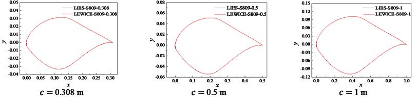
a) S809 airfoil
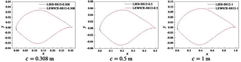
b) S812 airfoil
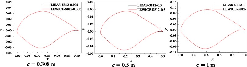
2.1.2. Linear interpolation with equiangular step (LIEAS)
A cartesian coordinate system was established as shown in Fig. 2, which takes the chord line of the unfrozen airfoil as the -axis and the midpoint of the line connecting the points M and N as the coordinate origin. Due to significant icing at the leading edge of the airfoil, the second quadrant was selected as an example for linear interpolation of the ice shape curve with equal angle steps (referred to as LIEAS) fitting. Linear interpolation with angle as a step size can effectively increase the number of key points describing the icing characteristics of the leading edge of the airfoil. The formula for ice interpolation key points is as follows:
where and are the coordinates of frost ice shape feature points before interpolation, are the coordinates of the point after interpolation, is the -th key point of the frost ice shape, and is the angle between the x axis and connection line of the interpolation point and coordinate origin.
Fig. 2Schematic diagram of LIEAS method
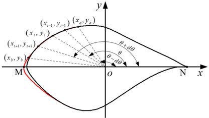
Fig. 3Fitting curves obtained by LIEAS method
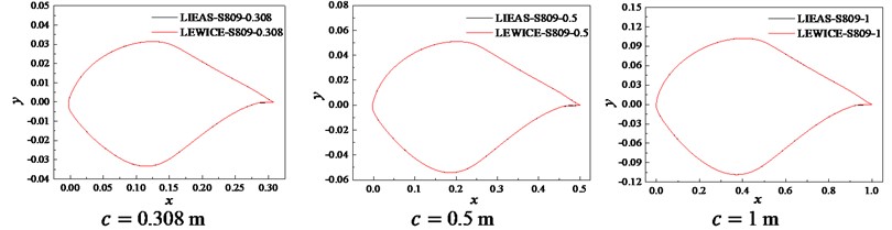
a) S809 airfoil
b) S812 airfoil
The frost ice shape curves of S809 and S812 airfoils were fitted by LIEAS method, as shown in Fig. 3. It can be seen from Fig. 3 that the most parts of ice shape obtained by LIEAS method are consistent with those simulated by LEWICE. However, the difference occurred in the rear edge icing zone. The difference in S812 airfoil is greater than that in S809. This is because the smaller trailing-edge angle and larger trailing-edge curvature on the lower surface make the ice shape feature points not interpolate. In general, the LIEAS method can fit the frost ice shape at the leading-edge very well, but there is a big difference at the trailing-edge on the lower surface.
2.1.3. Linear interpolation with equidistant and equiangular steps (LIEDEAS)
In view of the shortcomings of LIEDS and LIEAS methods, the LIEDEAS method was proposed to fit the frost ice shape of the airfoil. That is, the first and fourth quadrants used equal distance as the step size, while the second and third quadrants used equal angle as the step size. Fig. 4 shows that the frost ice shape fitting curves obtained by LIEDEAS method is highly consistent with those of LEWICE for S809 and S812 airfoils. The LIEDEAS method is suitable for the airfoil’s frost ice shape fitting, and establishes the foundation for the research on the blade’s frost ice shape formation method.
Fig. 4Fitting curves obtained by LIEDEAS method
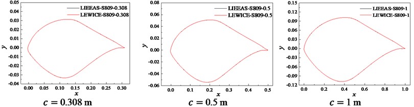
a) S809 airfoil
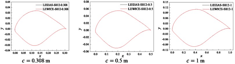
b) S812 airfoil
2.2. Verification of airfoil’s frost ice shape fitting method
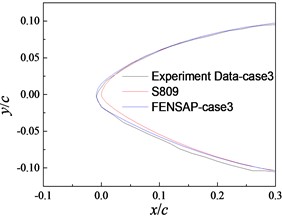
Compared the LIEDEAS results and FENSAP simulation results of the frost ice shape of the S809 airfoil with the experimental data in reference 12 to study the reliability of the two methods. Since the frost ice occurs mainly on the airfoil surface from the leading-edge to 0.3, the results in these areas were analyzed. Three frost ice conditions in Table 3 of Ref. 12 were selected, namely case 1, case 2 and case 3, as shown in Table 1.
Table 1Frost ice conditions
Frost ice | MVD (μm) | LWC (g/m3) | TEMP (°C) | Vel (m/s) | Time (min) | AOA (deg.) |
Case 1 | 20 | 0.08 | –4.5 | 50 | 30 | 2 |
Case 2 | 20 | 0.05 | –10 | 50 | 30 | 4 |
Case 3 | 20 | 0.05 | –9 | 50 | 30 | 4 |
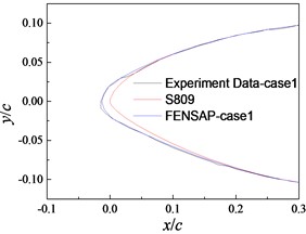
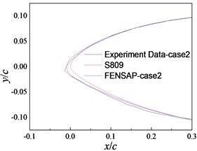
Fig. 5 gives the frost ice shapes from LIEDEAS method and experiments. In Fig. 5, the consistency between the results obtained by LIEDEAS method and experimental data is the best in case 1. The ice shapes from LIEDEAS method are similar to those of experiments except the frozen region of 0.1c-0.25c on the lower surface in case 2 and 3. Overall, the frost ice shapes obtained by LIEDEAS method are consistent with experimental results basically.
Fig. 5Comparison of frost ice shapes from LIEDEAS method and experiments
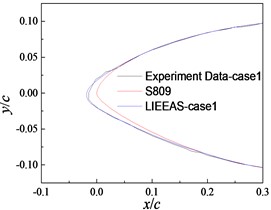
a) Case 1
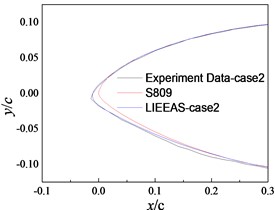
b) Case 2
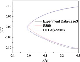
c) Case 3
The pre-processing software ICEM-CFD of FENSAP is used to generate the geometric model, calculation domain and grids of the equal-section blade with S809 airfoil, as shown in Fig. 6.
Fig. 6Calculation domain, symmetry surface indication and grids of equal-section blade
a) Calculation domain
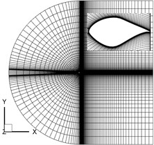
b) Symmetry surface indication
c) Grids
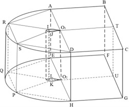
The blade and chord line are 0.5 m and 0.267 m in length, respectively. The calculation domain consisted of a semi-cylinder domain with a diameter of 50 and a height of 0.5 m, and a cuboid domain with a length of 50, a width of 25 and a height of 0.5 m. The trailing-edge was located on the axis of semi-cylinder. It was divided into 5 blocks, namely ARIO1O2EQL, IRSJKLQP, JSDO1O2KPH, O1DCTUGHO2 and O1TBAEO2UF, which were discretized using the structured grid. The grids were encrypted at the near wall, leading-edge and trailing-edge. For the edges AO1, DO1, EO2, HO2, BT, FU, CT, GU, RI, SJ, QL and PK, the division length at the end of the edge, the interval count and the successive ratio were specified. The Exponential 2 distribution law was used to perform the mesh division. For the edges SR, PQ, JI, KL, O2O1, KJ, LI, PS, QR, UT, GC, FB, EA and HD, the number of grid node and the division lengths at the start and end of the edge were specified. The successive ratio was calculated automatically by ICEM-CFD. The BiGeometric distribution law was used for the mesh division. For the edges RA, QE, PH, SD, IO1, JO1, LO2 and KO2, the number of grid node, the division lengths at the start and end of the edge, the successive ratio 1 (from the start to middle position) and the successive ratio 2 (from the end to middle position) were specified. The Biexponential distribution law was used for the mesh generation. For the edges O1T, AB, DC, EF, O2U and HG, the division length at the start of the edge, the interval count and the successive ratio 1 were specified. The Biexponential 1 distribution law was used for the mesh division. The grids of the equal-section blade consisted of 19,680 hexahedral elements and 39,892 nodes. The faces AEFB, ARSDHPQE, DHGC and CGFB were the velocity-inlet. The blade surfaces were no-slip and static-wall boundary conditions. The faces ARSDCB and EQPHGF were symmetrical boundaries -axisymmetry plane).
The .msh file of ICEM-CFD was imported into FENSAP to calculate the frost ice shape of the equal-section blade for case 1, 2, and 3, as shown in Fig. 7. Fig. 7 shows that the results of FENSAP are in good consistency with those of experiments in case 1, and there are some differences at the leading-edge and lower surface in case 2 and 3. The differences in case 3 are less for the leading-edge and greater for the lower surface than those in case 2, respectively. In a word, the differences in the ice shape are small between FENSAP and experiments.
Fig. 7Comparison of FENSAP and experiments results
a) Case 1
b) Case 2
c) Case 3
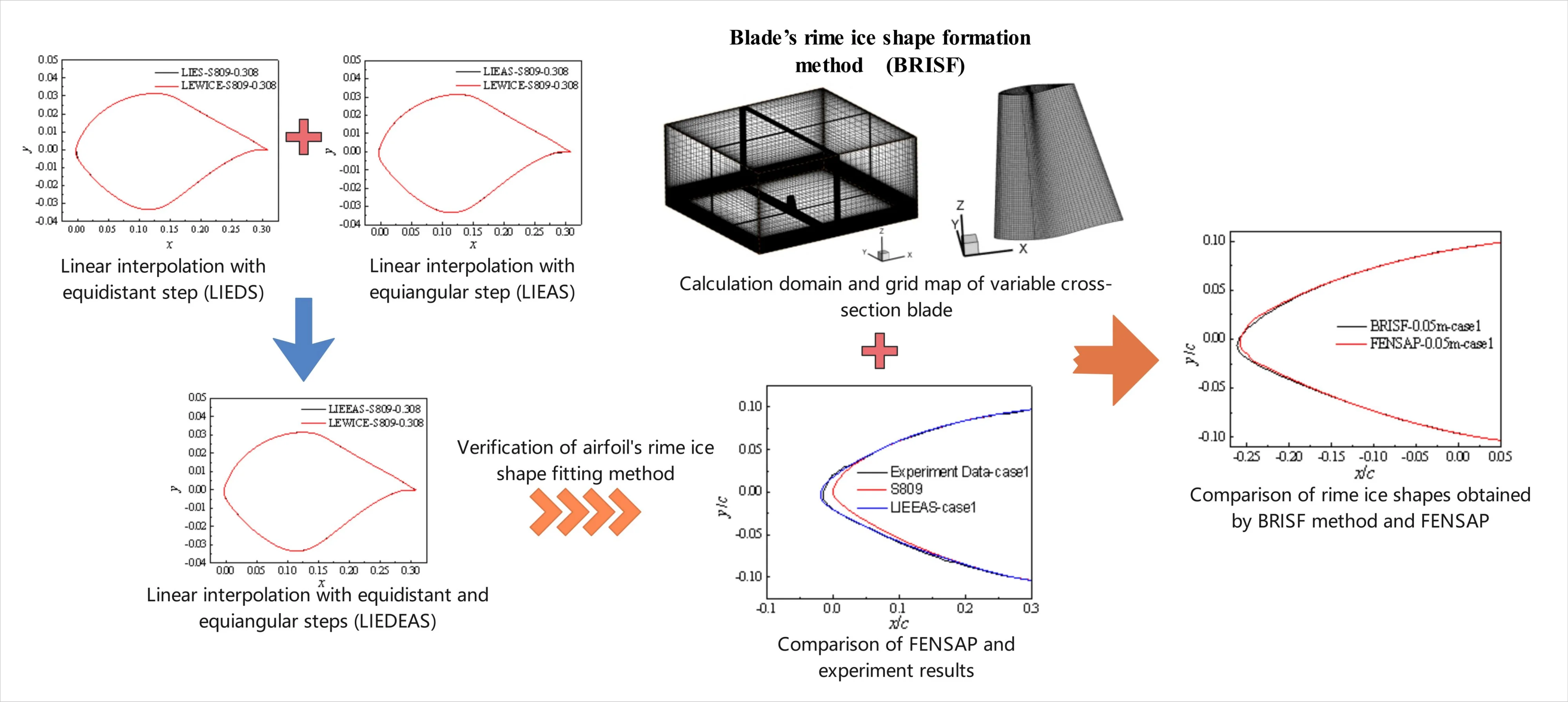
3. Blade’s frost ice shape formation method (BRISF)
The LIEDEAS method was used to fit the frost ice shapes of multiple sections along the span-wise direction to make the airfoil anywhere in the blade have the same number of ice shape feature points. The ice shape key point coordinates of adjacent sections were mapped into lagging and flapping surfaces by reducing the dimension, respectively. Then the polynomial fitting was applied to deal with projection points to form the space curve describing the frost ice shape.
The proposed blade frost ice formation method (BRISF) was applied to obtain the frost ice shape of S809 airfoil blades with variable chord length and twist angle in case 1, as shown in Fig. 8. The blade with evenly distributed 6 cross-sections along the span-wise direction is 0.5 m in length, and the chord length and torsion angle of the airfoil vary from 0.4 m to 0.233333 m and /180 to /1080, respectively.
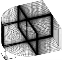
The geometric model, calculation domain and grids of the same blade were generated by ICEM-CFD, as shown in Fig. 9. The calculation domain was composed of a cuboid with 5.4 m long, 5 m wide and 5 m high. The blade was located in the center of the bottom surface. It was divided into 22 blocks, all of which were discretized using the structured grid. Block abcdefgh was the external O-Block of the blade. The length of the tail segment, the number of partitions, and the growth rate of unit height were defined. Exponential 2 was used to mesh edges E-l, E-4, E-8, and their parallel edges. Exponential distribution law Exponential1 was used to mesh edges E-2, E-3, E-6, and their parallel edges. Parabolic node distribution law BiGeometry was used to mesh edges E-5 E-7 and its parallel edges are meshed. The exponential distribution law was used to mesh E-9 and its parallel edges. The whole grid consists of 918,964 hexahedral elements and 886,050 nodes. The blade surface is static-wall and no-slip conditions. The faces ABCD, BCGF and FGHE are the velocity-inlet, and the faces ABFE and ADHE are the pressure-outlet. The CGHD face is symmetrical boundaries (-axisymmetry plane).
Fig. 8Blades with and without frost ice in case 1
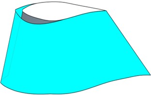
Fig. 9Calculation domain and grid map of variable cross-section blade
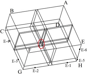
a) Calculation domain
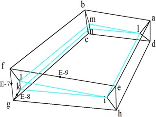
b) External O-Block of blade
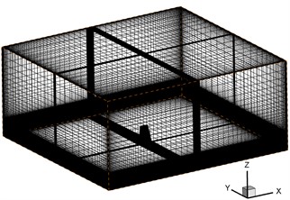
c) Mesh distribution around blade
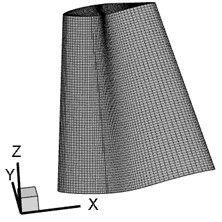
d) Grid map of blade
The frost ice shape of the variable cross-section blade was calculated through importing the .msh file of ICEM-CFD into FENSAP. It was compared with that of BRISF method for three cross-sections arbitrarily selected along span-wise direction, that is, 0.05 m, 0.245 m, and 0.376 m, as shown in Fig. 10. It can be seen from Fig. 10 that the ice shapes obtained by BRISF method are in good consistency with
FENSAP results in case 1, 2 and 3. There are some differences only at the leading-edge.
Fig. 10Comparison of frost ice shapes obtained by BRISF method and FENSAP
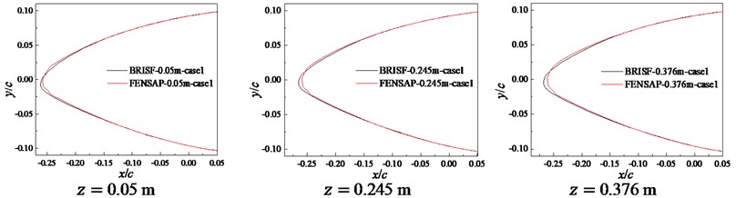
a) Case 1
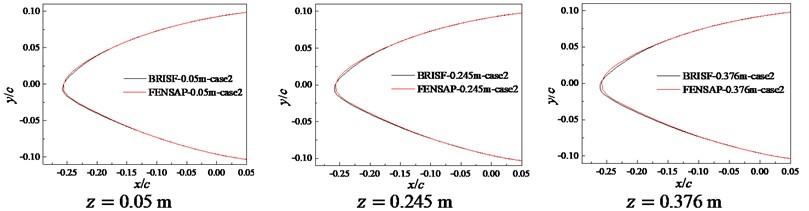
b) Case 2
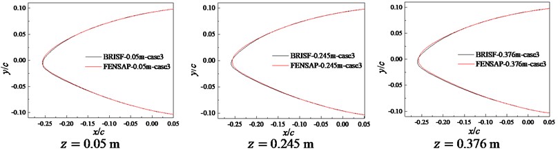
c) Case 3
4. Error analysis
In order to carry out a quantitative study on the errors of different numerical calculation methods of frost ice shapes for airfoils and blades, the residual sum of squares was used to analyze the differences between the LIEDEAS method and experiments, between the FENSAP simulation and experiments, and between the BRISF method and FENSAP simulation.
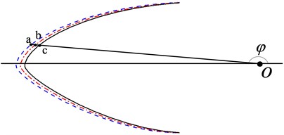
The chord of the unfrozen airfoil was used as the polar axis, and the midpoint of the chord was used as the pole. A polar coordinate system was established, as shown in Fig. 11. Lines oa, ob, and oc are the pole diameter at the same pole angle , which are the key points of frost ice shapes obtained by FENSAP, experiments and LIEDEAS method respectively. The polar diameters were used to calculate the residual sum of squares.
Fig. 11Polar diameters of frost ice shape key points from FENSAP, experiments and LIEDEAS method
The residual sum of squares on the upper and lower surfaces , , and the global residual sum of squares on the airfoil surface , , for frost ice shapes between LIEDEAS method and experiments, FENSAP and experiments, LIEDEAS method and FENSAP, respectively, are expressed as:
where is the number of key points of the frost ice shape before 0.3 on upper and lower surfaces, 1 and 2 is the upper and lower surfaces, and , and are the polar diameters of frost ice shapes from LIEDEAS method, FENSAP simulation and experiments, respectively.
4.1. Error analysis of airfoil’s frost ice shape fitting method
Table 2 gives the residual sum of squares of airfoil’s frost ice shape between LIEDEAS method and experiments, FENSAP simulation and experiments under different icing conditions. It is observed that the residual sum of squares on the upper, lower and airfoil surfaces are all the largest in case 3. But their orders of magnitude are still less than 10-3. This shows that the frost ice shapes obtained by LIEDEAS method and FENSAP simulation both coincide well with those of experiments, which are consistent with the analysis results of Fig. 5 and 7. It can also be seen that is smaller in case 1 and larger in case 2 and 3 than , respectively. The orders of magnitude of differences between and are all smaller than 10-4. So the proposed LIEDEAS method has the same accuracy and reliability of frost ice shape calculation with FENSAP.
Table 2Residual sum of squares of airfoil’s frost ice shapes obtained by different methods
Residual sum of squares | Icing conditions | ||
Case 1 | Case 2 | Case 3 | |
1.26E-04 | 6.63E-05 | 1.81E-04 | |
8.57E-05 | 1.22E-03 | 1.87E-03 | |
2.14E-04 | 1.28E-03 | 2.05E-03 | |
9.56E-05 | 1.45E-04 | 2.11E-04 | |
1.24E-04 | 7.54E-04 | 1.78E-03 | |
2.20E-04 | 8.89E-04 | 1.99E-03 | |
- | -6.67E-06 | 3.91E-04 | 6.00E-05 |
4.2. Error analysis of blade’s frost ice shape formation method
Table 3 gives the residual sum of squares of blade’s frost ice shape between BRISF method and FENSAP simulation on three cross-sections arbitrarily selected along the span-wise direction under different icing conditions. According to Table 3, , and are the largest in case 1 on three cross-sections, are the smallest in case 2 on the cross-section of 0.05 m, and are very close in case 2 and 3 on the two cross-sections of 0.245 m and 0.376 m, respectively. The orders of magnitude of , and are all less than 10-4. It can also be seen that the residual sum of squares on the upper, lower and airfoil surfaces are the smallest at the position of 0.05 m, and as the cross-sectional position approaches the blade tip, the sum of squared residuals increases. This indicates that the frost ice shape obtained by BRISF method near the blade root is in good coincide with that of FENSAP.
Table 3Residual sum of squares of blade’s frost ice shape between BRISF method and FENSAP
Cross-section | Icing conditions | |||
0.05 m | Case 1 | 6.87E-05 | 9.43E-05 | 1.63E-04 |
Case 2 | 3.23E-05 | 2.38E-05 | 5.60E-05 | |
Case 3 | 4.63E-05 | 2.65E-05 | 7.27E-05 | |
0.245 m | Case 1 | 1.17E-04 | 1.19E-04 | 2.36E-04 |
Case 2 | 5.67E-05 | 5.84E-05 | 1.15E-04 | |
Case 3 | 5.21E-05 | 5.81E-05 | 1.10E-04 | |
0.376 m | Case 1 | 1.71E-04 | 1.80E-04 | 3.51E-04 |
Case 2 | 9.18E-05 | 9.80E-05 | 1.90E-04 | |
Case 3 | 8.96E-05 | 9.85E-05 | 1.88E-04 |
5. Conclusions
The LIEDEAS method was used to fit the frost ice shape of the airfoil. The BRISF method was utilized to obtain blade frost ice shapes. Research the reliability of the proposed LIEEAS method and BRISF method from both qualitative and quantitative perspectives. The main conclusions are as follows:
1) Comparing and analyzing the ice shape results of the LIEDEAS method with experiments, it was found that the LIEDEAS method is suitable for ice shape fitting of any pointed or pure trailing edge airfoil. The obtained ice shape matches well with the experimental ice shape. Using FENSAP to simulate the frost ice shape of the S809 airfoil segment with equal cross-section, the obtained ice shape matches well with the experimental ice shape.
2) The proposed BRISF method was used to calculate the ice shape of S809 airfoil segments with variable chord length and twist angle under three operating conditions. Comparing the calculation results with the simulation results of FENSAP, the ice shape obtained by the two numerical methods has good consistency.
3) We calculated the sum of squared residuals of the upper, lower, and airfoil surfaces obtained from the LIEDEAS method and experiments. Their values are all small, and the sum of squared residuals corresponding to FENSAP and the experimental ice shape is not significantly different. The sum of squared residuals on the ice shaped upper and lower wing surfaces and airfoil surfaces of BRISF and FENSAP are relatively small. The order of magnitude is 10-4 or 10-5, which is less than the sum of squared residuals of FENSAP simulation and experimental results for airfoil frost ice shapes. The new method has high accuracy.
References
-
G. Botta, M. Cavaliere, S. Viani, and S. Pospı́šil, “Effects of hostile terrains on wind turbine performances and loads: The Acqua Spruzza experience,” Journal of Wind Engineering and Industrial Aerodynamics, Vol. 74-76, pp. 419–431, Apr. 1998, https://doi.org/10.1016/s0167-6105(98)00038-5
-
M. Etemaddar, M. O. L. Hansen, and T. Moan, “Wind turbine aerodynamic response under atmospheric icing conditions,” Wind Energy, Vol. 17, No. 2, pp. 241–265, Nov. 2012, https://doi.org/10.1002/we.1573
-
B. Xu, F. Lu, and G. Song, “Experimental study on anti-icing and deicing for model wind turbine blades with continuous carbon fiber sheets,” Journal of Cold Regions Engineering, Vol. 32, No. 1, pp. 1–10, Mar. 2018, https://doi.org/10.1061/(asce)cr.1943-5495.0000150
-
L. Hu, X. Zhu, C. Hu, J. Chen, and Z. Du, “Wind turbines ice distribution and load response under icing conditions,” Renewable Energy, Vol. 113, pp. 608–619, Dec. 2017, https://doi.org/10.1016/j.renene.2017.05.059
-
M. C. Homola, M. S. Virk, P. J. Nicklasson, and P. A. Sundsbø, “Performance losses due to ice accretion for a 5 MW wind turbine,” in Wind Energy, Vol. 15, No. 3, pp. 379–389, Jun. 2011, https://doi.org/10.1002/we.477
-
X. Yi, G. L. Zhu, K. C. Wang, and Y. W. Gui, “Selection of water droplet diameter in icing wind tunnel test,” (in Chinese), Acta Aeronautica Et Astronautica Sinica, Vol. 31, No. 5, pp. 877–882, 2010.
-
X. Yi, Y. W. Gui, and G. L. Zhu, “Numerical method of a three-dimensional ice accretion model of aircraft,” (in Chinese), Journal of Aircraft, Vol. 31, No. 11, pp. 2152–2158, 2010.
-
W. J. Jasinski, S. C. Noe, M. S. Selig, and M. B. Bragg, “Wind turbine performance under icing conditions,” Journal of Solar Energy Engineering, Vol. 120, No. 1, pp. 60–65, Feb. 1998, https://doi.org/10.1115/1.2888048
-
J. Shin and T. Bond, “Results of an icing test on a NACA 0012 airfoil in the NASA Lewis Icing Research Tunnel,” in 30th Aerospace Sciences Meeting and Exhibit, pp. 1–23, Jan. 1992, https://doi.org/10.2514/6.1992-647
-
Y. Han, J. Palacios, and S. Schmitz, “Scaled ice accretion experiments on a rotating wind turbine blade,” Journal of Wind Engineering and Industrial Aerodynamics, Vol. 109, pp. 55–67, Oct. 2012, https://doi.org/10.1016/j.jweia.2012.06.001
-
A. G. Kraj and E. L. Bibeau, “Phases of icing on wind turbine blades characterized by ice accumulation,” Renewable Energy, Vol. 35, No. 5, pp. 966–972, May 2010, https://doi.org/10.1016/j.renene.2009.09.013
-
Y. Li, F. Feng, S. M. Li, W. Q. Tian, and K. Tagawa, “Wind tunnel test on icing on a straight blade for vertical axis wind turbine,” Advanced Materials Research, Vol. 301-303, No. 11, pp. 1735–1739, Jul. 2011, https://doi.org/10.4028/www.scientific.net/amr.301-303.1735
-
S. M. Li, “Studies on icing effect on aerodynamics characteristics of the straight-bladed vertical axis wind turbine,” (in Chinese), Northeast Agricultural University, Harbin, China, 2011.
-
O. Yirtici, I. H. Tuncer, and S. Ozgen, “Ice accretion prediction on wind turbines and consequent power losses,” Journal of Physics: Conference Series, Vol. 753, No. 2, p. 022022, Sep. 2016, https://doi.org/10.1088/1742-6596/753/2/022022
-
M. Brahimi, D. Chocron, and I. Paraschivoiu, “Prediction of ice accretion and performance degradation of HAWT in cold climates,” in 1998 ASME Wind Energy Symposium, pp. 60–69, Jan. 1998, https://doi.org/10.2514/6.1998-26
-
G. M. Ibrahim, K. Pope, and Y. S. Muzychka, “Effects of blade design on ice accretion for horizontal axis wind turbines,” Journal of Wind Engineering and Industrial Aerodynamics, Vol. 173, pp. 39–52, Feb. 2018, https://doi.org/10.1016/j.jweia.2017.11.024
-
Muhammad S. Virk, Matthew C. Homola, and Per J. Nicklasson, “Atmospheric icing on large wind turbine blades,” International Journal of Energy and Environmental Engineering, Vol. 3, No. 1, pp. 1–8, Jan. 2012.
-
T. Hedde and D. Guffond, “ONERA three-dimensional icing model,” AIAA Journal, Vol. 33, No. 6, pp. 1038–1045, Jun. 1995, https://doi.org/10.2514/3.12795
-
P. Fu and M. Farzaneh, “A CFD approach for modeling the rime-ice accretion process on a horizontal-axis wind turbine,” Journal of Wind Engineering and Industrial Aerodynamics, Vol. 98, No. 4-5, pp. 181–188, Apr. 2010, https://doi.org/10.1016/j.jweia.2009.10.014
-
J. Liang, L. C. Shu, Q. Hu, X. L. Jiang, G. H. He, and Y. Liu, “3-D numerical simulations and experiments on glaze ice accretion of wind turbine blades,” (in Chinese), Proceedings of the CSEE, Vol. 37, No. 15, pp. 4430–4436, 4584, https://doi.org/10.13334/j.0258-8013.pcsee.161239
-
X. Yi, K. C. Wang, H. L. Ma, and G. L. Zhu, “Computation of icing and its effect of horizontal axis wind turbine,” (in Chinese), Acta Energiae Solaris Sinica, Vol. 35, No. 6, pp. 1052–1058, 2014.
-
X. H. Deng, “Numerical simulation of ice accretion process on horizontal-axis wind turbine blade,” (in Chinese), Changsha University of Science and technology, Changsha, China, 2011.
-
W. Jiang, Y. D. Li, H. B. Li, X. H. Deng, and Y. X. Liu, “Simulation of icing on horizontal-axis wind turbine blade,” (in Chinese), Acta Energiae Solaris Sinica, Vol. 35, No. 1, pp. 83–88, 2014.
-
A. Zanon, M. de Gennaro, and H. Kühnelt, “Wind energy harnessing of the NREL 5 MW reference wind turbine in icing conditions under different operational strategies,” Renewable Energy, Vol. 115, pp. 760–772, Jan. 2018, https://doi.org/10.1016/j.renene.2017.08.076
-
C. Hochart, G. Fortin, J. Perron, and A. Ilinca, “Wind turbine performance under icing conditions,” Wind Energy, Vol. 11, No. 4, pp. 319–333, Oct. 2007, https://doi.org/10.1002/we.258
-
M. Dimitrova, D. Ramdenee, and A. Ilincs, “Evaluation and mitigation of ice accretion effects on wind turbine blades,” in World Renewable Energy Congress, 2011.
-
T. Reid, G. Baruzzi, I. Ozcer, D. Switchenko, and W. Habashi, “FENSAP-ice simulation of icing on wind turbine blades, part 1: performance degradation,” in 51st AIAA Aerospace Sciences Meeting including the New Horizons Forum and Aerospace Exposition, Jan. 2013, https://doi.org/10.2514/6.2013-750
About this article

This work was supported by the Science and Technology Planning Project of Tianjin, China (Grant No. 20YDTPJC00820), and Natural Science Basic Research Program of Shaanxi, China (Program No. 2022JM-252).
The datasets generated during and/or analyzed during the current study are available from the corresponding author on reasonable request.
Renfeng Zhang: software, supervision, review and editing. Gege Wang: data curation, software, original draft preparation, writing. Xin Wang: supervision.
The authors declare that they have no conflict of interest.
