Abstract
When the current transfer learning algorithm is applied to the field of bearing fault diagnosis under different working conditions, it only focuses on reducing the cross-domain distance or the distribution difference within the domain, and does not consider the domain tilt. When the fault samples are scarce, the degradation of recognition ability is more obvious. A fault diagnosis method for rolling bearings based on cross-domain divergence alignment and intra-domain distribution alienation (CDDA-IDDA) is proposed. Firstly, aiming at the cross-domain tilt in the domain data space of variable working conditions, the overall divergence matrix of source domain and target domain is constructed, and the cross-domain divergence alignment is carried out. Then, aiming at the overlapping phenomenon of categories in the domain, based on the distribution adaptation weighted conditional distribution, the spatial distribution of different categories in the same domain is further alienated. Finally, the regularization term is introduced under the framework of structural risk minimization. On the basis of fully retaining the internal structure of the data, a multi-classifier with strong transfer ability is obtained by iteration. Experiments show that the proposed method is better than some mainstream transfer learning algorithms in multi-fault, multi-degree recognition and compound fault diagnosis. In addition, the proposed method still has high diagnostic accuracy when there are few labeled training samples. When the ratio of labeled source domain samples to unlabeled target domain is 1:50 (16 labeled data), the average accuracy of the transfer task reaches 97.78 %.
Highlights
- Regularized within-class scatter matrix is proposed.
- The cross-domain tilt problem is solved in the subspace by the regularized overall divergence matrix.
- The weighted conditional distribution is used to fit the distance of the same type of samples across the domain and reduce the overlap of fault categories within the domain.
- Under the framework of structural risk minimization, a multi-classifier with strong transfer ability is obtained.
1. Introduction
As an indispensable part of modern industrial production, the accidental failure of bearings may cause huge economic losses and even endanger people's lives. With the increasing complexity of mechanical equipment, the acquisition of equipment status information has become more and more difficult. The amount of fault data is small, and the label samples are very precious [1]. If only rare fault data is used to learn the diagnosis model, it will lead to poor model performance and low fault classification accuracy. Therefore, in order to make efficient use of existing fault data, improve the fault diagnosis ability under small samples, fully exploit the similarity between data, and improve the generalization ability of the model becomes very important.
At present, the fault diagnosis process of rolling bearings is mainly divided into three parts: vibration signal acquisition, feature extraction and fault identification. Among them, there are many traditional fault classification methods, such as K-nearest neighbor (KNN), support vector machine (SVM), random forest (RF), and so on. However, most of the existing machine learning methods are based on two basic premises: 1) The distribution of training data and test data is the same; 2) Enough available training samples [5]. Only by satisfying these two conditions can a good diagnostic model be learned.
Data distribution requires the same environmental conditions when collecting bearing vibration signals. However, with the increasing complexity of mechanical equipment, the installation of vibration signal sensors is becoming more and more diversified, which leads to the increasing difference in the distribution of bearing vibration signals at different acquisition positions. Traditional fault diagnosis algorithms are often ineffective [6]. In the context of the Internet of Things and big data, most machine learning will collect data in various parts of the machine equipment that may fail, [7] and train multiple fault diagnosis models. This method can also solve the problem of different distribution of data, but it will consume huge manpower and material resources and is expensive. Transfer learning emerges as the times require. Transfer existing knowledge to solve the learning problem that label samples are difficult to obtain in the target domain. The method of applying the knowledge learned in a certain domain (source domain) to different but related domains (target domain) is called transfer learning [8]. Transfer learning also has many applications in the field of fault bearing fault diagnosis [9-11]. Considering that similar fault characteristics will appear in bearing vibration data under variable working conditions, cross-domain distribution adaptation has become a hot issue to be solved in the field of bearing fault diagnosis. Lan et al. [12] proposed a cross-domain bearing fault classification method based on transfer component analysis (TCA). By minimizing the maximum mean difference between the source domain and the target domain, the distribution distance between the domains is significantly reduced to achieve cross-domain marginal distribution alignment. Chen et al. [13] used Geodesic flow kernel (GFK) combined with source domain multiple samples to fully mine source domain sample information, which improved the recognition accuracy of rolling bearing life state under different working conditions. Manifold Embedded Distribution Alignment (MEDA) is a transfer manifold learning method with dynamic distribution adaptive ability proposed by Wang et al. [14] on the basis of Joint Distribution Adaptation (JDA) [15]. It achieves better domain adaptation by quantitatively evaluating the relative importance of marginal distribution and conditional distribution. Zhang et al. [16] proposed a small sample bearing fault diagnosis method based on transfer learning, using a sufficient number of source domain samples to train the network to prevent network overfitting, and using 1 % target domain training set data to fine-tune the model classification ability. Zhao et al. [17] used bidirectional gated recurrent units to generate auxiliary samples for the source domain of MEDA, so that excellent fault identification can be maintained in the case of a small number of labeled samples. The above research focuses on the alignment of marginal distribution and conditional distribution. As a cross-domain alignment, these two distribution alignments aim to reduce the distance between the source domain and the target domain, ignoring the possibility of spatial tilt of the domain and ignoring the internal structure information of the domain, which may lead to the overlap of categories in the domain. Considering the differences in the internal distribution of the domain, many scholars have studied this problem, such as Cao et al. [18] projection maximum local weighted deviation, which reflects the global distribution difference through the difference in the distribution of local subdomains, reflects the local distribution difference between the source domain and the target domain, and has achieved good results on face recognition data. However, the possibility of domain skew is not considered, and the performance is unknown under small samples. In the case of small samples, the common solution is to use a small number of existing samples to generate auxiliary training samples, or to use a small number of target samples to adjust the model. It does not fundamentally solve the learning ability of the model in small samples, and the generation of auxiliary samples will increase the algorithm’s time complexity. In order to establish a connection between the source domain and the target domain, the structural information in the domain is transmitted across the domain to avoid the distribution distance between the classes in the domain is too small, and the adaptability of the algorithm under small samples is improved. Therefore, this paper proposes a rolling bearing transfer fault diagnosis method based on cross-domain divergence alignment and intra-domain distribution alienation. Firstly, the inter-class divergence matrix and the regularized intra-class divergence matrix of the source domain and the target domain are constructed respectively to form the overall divergence matrix, and the cross-domain divergence alignment is performed on the subspace to solve the cross-domain tilt problem. Then, on the basis of the weighted conditional distribution adapting to the same type of sample distance between the source domain and the target domain, the spatial distribution of different categories in the same domain is further alienated, and the intra-domain structure is adjusted so that the error between the predicted label and the real label can be gradually reduced in the iteration while reducing the overlap of categories in the domain. Finally, under the framework of structural risk minimization, the regularization term is introduced to fully retain the internal structure of the data, and the multi-classifier with strong transfer ability is obtained.
2. Transfer learning algorithm based on cross-domain divergence alignment and intra-domain distribution alienation
Due to the difference in the spatial distribution of the source domain and the target domain, simple feature normalization in the domain cannot solve the domain offset problem. When the sample size of the source domain is scarce, the effect of aligning the source domain and the target domain often decreases significantly, and the existing transfer learning methods pay more attention to the minimization of cross-domain distance and pay little attention to the distribution within the domain when performing domain adaptation. Therefore, a transfer learning method based on cross-domain divergence alignment and intra-domain distribution alienation is proposed to eliminate the phenomenon of domain offset and intra-domain overlap and improve the effect of cross-domain alignment under small samples.
2.1. Subspace cross-domain divergence alignment subspace alignment
The subspace learning method usually assumes that the data in the source domain and the target domain will have similar distribution in the transformed subspace. In general, since the source domain and the target domain sample data acquisition environment are different, it is assumed that they are in different subspaces, and often similar matrices will lead to similar distributions [19]. Therefore, we need to align the domain data matrix in the appropriate subspace, assuming that there is a sample data with known labels as the source domain, and a sample data with unknown labels as the target domain, where, , , is the dimension of signal. The purpose of subspace alignment is to find a transformation matrix and transform the source domain data into a subspace that can be aligned with the target domain data. The following optimization objective function can be obtained:
where represents the Frobenius norm. Learning the transformation matrix makes the source domain data adapt to the target domain data , so that the two domain data are as similar as possible. Solving matrix requires that the number of samples in the two domains is equal, that is, . However, due to the differences in the environment in which the samples are located, the difficulty of sample acquisition is also inconsistent, so it is difficult to ensure that the two domain data are equal.
In order to solve this problem, we use the overall divergence matrix in the domain to replace the samples in the domain, which can not only ensure the equal dimension of the two domains, but also mine the class structure in the domain.
2.2. Overall divergence
Suppose that denotes the center point of class in the domain, denotes the center point of the whole domain, denotes the number of samples in class , and denotes the sample set of class . The calculation equations of between-class scatter matrix , within-class scatter matrix and overall scatter matrix can be obtained:
where is the regularization parameter and is the diagonal matrix of the matrix.
2.3. Cross-domain divergence alignment
In order to better align the source domain and the target domain in the subspace and perform cross-domain transfer of the intra-domain structure, this paper implements subspace divergence alignment by embedding the overall divergence matrix of the source domain and the target domain in the subspace to reduce the domain space offset. Since the target domain sample data is unlabeled, it is necessary to first use the source domain label data to train a KNN classifier to obtain the pseudo label of the target domain. Assuming that and are the overall divergence matrices of the source domain and the target domain, respectively, and the transformation matrix is , the divergence alignment process can be expressed as:
Thus, it can be derived from Eq. (5):
Therefore, an optimization result can be obtained. When the overall divergence matrix of the source domain cannot be inverted, its Moore-Penrose pseudo-inverse can be used to correct the linear transformation matrix . Finally, we get the new source domain sample data after divergence alignment.
2.4. Inter-domain weighted conditional distribution alignment
The above divergence cross-domain alignment is equivalent to the overall alignment of domain data and the transmission of intra-domain information. It does not minimize the distance between cross-domain samples of the same class. Therefore, it is necessary to adapt the conditional distribution between domains to minimize the distance between samples of the same class in the source domain and the target domain.
In feature-based transfer learning, Maximum Mean Discrepancy (MMD) is often used to measure the cross-domain feature distribution. The conditional distribution based on the maximum mean difference is usually expressed as:
Among them, is the feature space, represents the reproducing kernel Hilbert space (RKHS), is the number of samples belonging to class in the source domain, and is the number of samples belonging to class in the target domain.
However, in the actual convergence process of the classifier, the target domain uses pseudo labels obtained by the weak classifier. Even if the number ratio of the same class in the source domain and the target domain is the same in practice, in the process of iteration, due to the error between the source domain and the real label, the same class ratio of the two domains will be different [21]. In the process of conditional distribution adaptation, the weight of each class is added, and the weighted conditional maximum mean difference is used to replace the original conditional distribution difference. The expression is as follows:
where, and represent the weight coefficients of class samples in the source domain and the target domain, respectively, calculated by , and represents the prior probability of class .
2.5. Distribution alienation between classes within the domain
In order to further mine the intra-domain structure information and retain the intra-domain label distribution difference, the label distribution distance between the source domain and the target domain is adjusted. Similarly, this paper uses the mean difference of the maximum mean difference in the Hilbert space of the reproducing kernel to represent the distance between the classes in the domain, and obtains the distribution distance between the source domain and the target domain:
where, is the feature space; represents the reproducing kernel Hilbert space (RKHS); and are the number of samples belonging to class and non-class in the source domain, respectively. , similarly; is the total number of categories.
Since the inter-class distribution in the source domain uses real labels, the labels will not change during the iteration process, while the inter-class distribution in the target domain uses pseudo labels obtained by the weak classifier (KNN). Therefore, it is only necessary to introduce weighting coefficients into the inter-class distribution distance of the target domain to obtain:
where, and represent the weight coefficients of the target domain class and non-class respectively, and , , and represent the prior probabilities of the source domain class and non-class respectively.
2.6. An optimal classifier is constructed based on structural risk minimization
According to the representation theorem [22], the classifier can be expressed as:
Given a Hilbert space and a kernel function , the structure risk function of the mapping from the original space to the Hilbert space is as follows:
where, is the classifier in kernel space, is the label of , is the square norm, is the regularization parameter, and the classifier with low expected error is obtained by minimizing the structural risk function. The final classifier is expressed as:
where, is the inter-domain weighted conditional distribution term, is the source domain inter-class distribution alienation term, is the target domain weighted inter-class distribution alienation term, is the regularization parameter, and is the Laplace regularization term, which is used to further mine the geometric similarity in the data space and ensure that there is no over-fitting in the iterative process. It is expressed as:
The pairwise similarity matrix is expressed as:
where is a similarity function, and is the nearest neighbor set of point . By calculating the Laplacian matrix , where is the diagonal matrix of the similar matrix , the regularization is finally obtained.
Then, according to the representation theorem and kernel technique, the classifier function is transformed into:
where, is the label matrix predicted according to the label information of the source domain. represents the trace of the matrix. , , and represent the diagonal indicator matrix, the inter-domain weighted conditional distribution matrix of class , and the intra-domain distribution matrix of the source domain and the target domain, respectively. It can be calculated:
Let the partial derivative , get the optimal solution:
where, is the unit matrix, is the kernel matrix, , and , and the optimal classifier is obtained by replacing the Eq. (22) with the Eq. (12).
3. Rolling bearing fault diagnosis model based on cross-domain divergence alignment and intra-domain distribution alienation
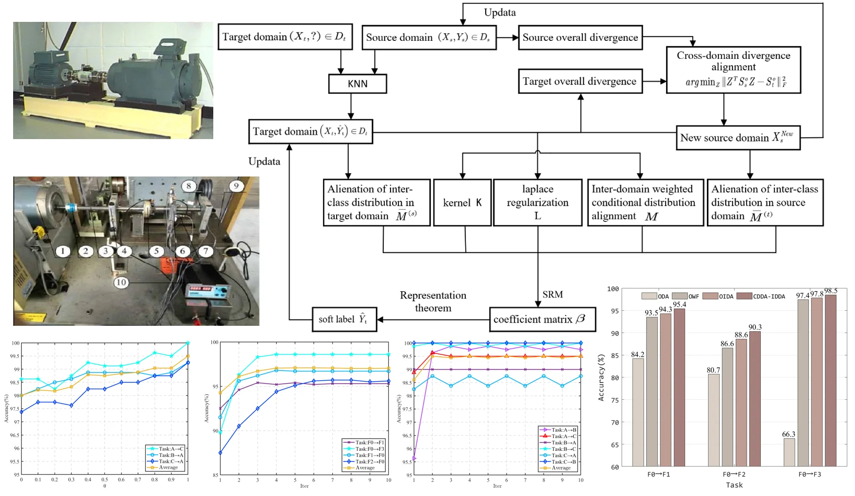
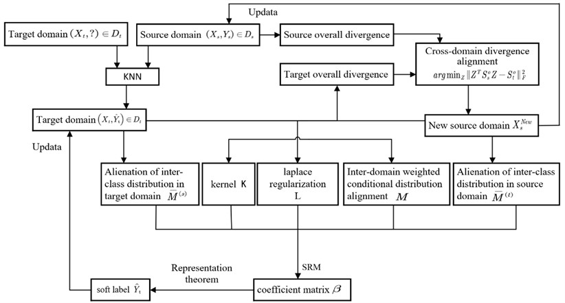
Based on cross-domain divergence alignment and intra-domain distribution alienation method, the fault diagnosis of rolling bearings under variable working conditions is carried out. Firstly, the labeled source domain samples are used to train the KNN model to obtain pseudo-labels for the unlabeled target domain. The overall divergence matrices of the source domain and the target domain are constructed respectively for cross-domain divergence alignment. Then, on the basis of adaptive weighted conditional distribution, the spatial distribution between categories in the domain is further alienated, and the overlap of categories in the domain is effectively reduced. Finally, a fault diagnosis model is constructed under the framework of minimizing structural risk. The overall process of fault diagnosis proposed in this paper is shown in Fig. 1. The specific process can be divided into the following six steps:
Step 1: The bearing vibration signal of the known label is taken as the source domain , and the signal data of the unknown label is taken as the target domain . The vibration signal samples in the source domain and the target domain are extracted as input.
Step 2: uses the labeled source domain data to train a weak classifier (KNN) to obtain the target domain pseudo-label .
Step 3: Divergence alignment: According to the source domain sample and the target domain sample , the between-class divergence matrix and the within-class divergence matrix are calculated respectively, and the overall divergence matrix and of the source domain and the target domain are constructed by Eq. (4). The intra-domain divergence matrix is embedded in the subspace optimization objective function for cross-domain divergence alignment, and a new optimization objective function is obtained: . According to the linear transformation matrix derived from the objective function, the original source domain data can be transformed to obtain the new source domain data after divergence alignment.
Step 4: Weighted conditional distribution adaptation: The cross-domain weighted conditional distribution adaptation can be expressed as: by the maximum mean difference function and kernel technique. In this process, the prior probability of class is calculated according to the number of samples in each class, and the conditional distribution matrix of class is calculated according to the Eq. (19), and all conditional distribution matrices are obtained.
Step 5: Alienation of inter-class distribution in the domain: Similarly, the inter-class distribution alienation terms of the source domain and the target domain are transformed into the form of matrix traces: and , and the prior probability of class in the target domain is calculated. According to Eq. (20) and Eq. (21), the maximum mean difference matrices and of class in the source domain and the target domain are calculated, and the total distribution matrices and are obtained by summing.
Step 6: Calculate the Laplacian regularization matrix and the kernel matrix , obtain the optimal solution according to Eq. (22), it back to Eq. (12) to obtain the classifier . Use this classifier to update the target domain pseudo-label , repeat steps 3 to Step 6 until the result converges.
Fig. 1Overall process of fault diagnosis
4. Experimental verification
4.1. Different working condition bearing fault diagnosis experiment
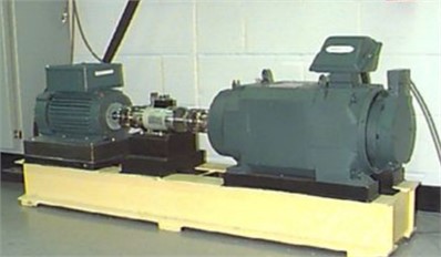
In this paper, the open bearing vibration data set of Case Western Reserve University (CWRU) is used to verify the bearing fault diagnosis algorithm. The test device is shown in Fig. 2. The left side is a 2 horsepower three-phase induction motor, and the right side is a dynamometer for generating rated load. The two are aligned through a torque sensor. The measured object is a deep groove ball bearing installed at the motor drive end, and the vibration sensor is installed on the upper side of the motor drive end.
Fig. 2CWRU bearing experimental device
The selected data has four health type: normal (NO), inner ring fault (IF), ball fault (BF), outer ring fault (OF). Each of the three fault states has three fault sizes (0.007', 0.014', 0.0021') and four motor conditions (0 HP/1797 rpm, 1 HP/1772 rpm, 2 HP/1750 rpm, 3 HP/1730 rpm). The sampling frequency is 12 KHZ.
In this paper, the transfer task of bearings under different working conditions is set up. The bearing vibration data of any working condition is taken to construct the source domain sample set, and the data of another different working condition is taken to construct the target domain sample set, so as to simulate the bearing fault type identification under variable working conditions in practice. Among them, each health status has 100 samples, each sample contains 2048 data points, and each sample set has a total of 1000 samples. The data set is marked to obtain 4 sample sets, and two different data sets constitute a transfer task, so that 12 transfer tasks of variable condition fault diagnosis can be obtained. The data set is shown in Table 1.
Table 1Description of bearing data set
Data set | Working conditions | Number of samples | class |
F0 | 0 HP/1797 rpm | 1000 | 10 |
F1 | 1 HP/1772 rpm | 1000 | 10 |
F2 | 2 HP/1750 rpm | 1000 | 10 |
F3 | 3 HP/1730 rpm | 1000 | 10 |
Table 2Bearing data set type description
Label | Type | Label | Type |
1 | NO | 6 | BF 0.014" |
2 | IF 0.007" | 7 | OF 0.014" |
3 | BF 0.007" | 8 | IF 0.021" |
4 | OF 0.007" | 9 | BF 0.021" |
5 | IF 0.014" | 10 | OF 0.021" |
4.2. Different working condition small sample bearing composite fault diagnosis experiment
In order to verify that the proposed method not only has better recognition ability on the public bearing fault data set, but also has better performance on other bearing composite fault data sets, and when the training samples are insufficient, it also reflects excellent generalization ability. The performance of the proposed method is evaluated by comparing it with several most popular transfer learning methods.
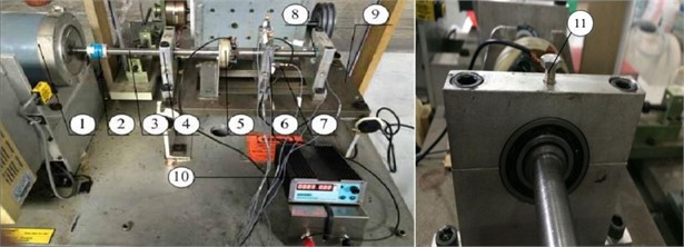
In this paper, the simulation experiment platform of bearing compound fault is shown in Fig. 3. The test bearing of this experiment is a detachable deep groove ball bearing, its model is 6205EKA. Three different working conditions (500 N/1800 rpm, 1000 N/1200 rpm, 1500 N/600 rpm) were set up in the experiment, and the sampling frequency was 16384HZ. The selected data have eight health states: normal (NO), outer ring fault (OF), inner ring fault (IF), ball fault (BF), inner ring + ball fault (IF+BF), outer ring + inner ring fault (IF+OF), outer ring + ball fault (OF+BF), outer ring + inner ring + ball fault (IF+OF+BF). Among them, each health type has 100 samples, each sample contains 2048 data points, and each sample set has a total of 800 samples. The data set is marked to obtain a sample set of three different working conditions, and the two data sets constitute a transfer task, so that six transfer tasks of different working condition fault diagnosis can be obtained.
Fig. 3Bearing compound fault test bench: 1 – motor; 2 – coupling; 3 – spindle; 4 – bearing housing; 5 – carbon brush; 6 – test bearing housing; 7 – vibration acceleration sensor; 8 – bearing; 9 – base; 10 – power; 11 – load bolts
At the same time, this paper sets the bearing compound fault identification task of small sample training set under different working conditions: take the bearing vibration data of any working condition, randomly select N samples from 100 samples of each bearing type, so as to construct the source domain small sample set, and take all the data of another different working condition to construct the target domain sample set, so as to simulate the actual small sample under the bearing variable condition compound fault type identification.
The data set description is shown in Table 3 and Table 4.
Table 3Description of bearing composite fault data set
Data set | Working conditions | Number of samples | Class |
A | 500 N/1800 rpm | 800 | 8 |
B | 1000 N/1200 rpm | 800 | 8 |
C | 1500 N/600 rpm | 800 | 8 |
Table 4Description of bearing data set type
Label | Type | Label | Type |
1 | NO | 5 | IF+BF |
2 | OF | 6 | IF+OF |
3 | IF | 7 | OF+BF |
4 | BF | 8 | IF+OF+BF |
5. Experimental result
5.1. Experimental results of different working condition bearing
In order to demonstrate the effectiveness of the proposed method, the proposed method is compared with other machine learning algorithms, five mainstream transfer learning methods and a typical traditional algorithm, as follows:
SVM: A common baseline method in classification tasks.
BDA [21]: Weighted joint distribution adaptation method.
GFK [23]: Manifold feature learning method, marginal distribution adaptation on Grassmann manifold.
TCA [24]: Marginal distribution adaptation method.
JDA [15]: Joint marginal distribution and conditional distribution adaptation method.
MEDA [14]: Manifold embedded adaptive distribution adaptation method, which can dynamically change the weight of marginal distribution and conditional distribution.
Among them, GFK and TCA belong to the marginal distribution alignment method; BDA, JDA and MEDA are joint distribution adaptation methods that consider both marginal distribution and conditional distribution.
The transfer learning methods all use the KNN algorithm to obtain weak labels for the target domain, and the subspace dimension d is set to 5. The regularization parameter in this algorithm is set to 0.9; the parameters and were set to 10 according to reference [14]. The parameters , and are set by traversing –1 to 1 interval of 0.1, and finally determined as 0.1, = –0.1 and 0.1; the number of iterations 10; the same hyperparameters involved in the other algorithms are set to the same value.
The bearing fault diagnosis results of seven classification algorithms under different transfer tasks are obtained, as shown in Table 5.
It can be seen from the table that the recognition rate of all tasks on the CWRU dataset is higher than that of other algorithms. The reason is that the two sets of data with different working conditions have different spaces. The method in this paper fully considers the divergence offset of inter-domain data, aligns the data divergence, and then further mines the distribution structure in the domain, adjusts the inter-class distance, and introduces the weighting factor to align the distribution, which effectively avoids the feature distortion, and can continuously adjust the spatial distribution of the data through iteration. The results show that the proposed method has good performance in the recognition accuracy of multi-fault size and multi-fault type under different working conditions. It is 5.34 % higher than the most widely used transfer learning method MEDA, and the standard deviation is the lowest, which proves the stability of the algorithm.
Table 5Accuracy of bearing fault identification under different working conditions by different methods
Task | SVM | BDA | GFK | TCA | JDA | MEDA | CDDA-IDDA |
F0→F1 | 87.2 | 91.0 | 91.0 | 82.4 | 91.4 | 87.8 | 95.4 |
F0→F2 | 85.5 | 89.9 | 77.6 | 85.3 | 86.0 | 86.5 | 90.3 |
F0→F3 | 88.6 | 93.8 | 81.0 | 85.5 | 90.1 | 85.2 | 98.5 |
F1→F0 | 87.1 | 90.6 | 89.0 | 75.9 | 89.3 | 91.9 | 96.7 |
F1→F2 | 98.8 | 89.5 | 86.4 | 96.2 | 89.2 | 90.4 | 98.9 |
F1→F3 | 97.3 | 94.9 | 87.2 | 94.7 | 92.7 | 95.0 | 99.4 |
F2→F0 | 89.7 | 84.0 | 72.5 | 84.7 | 87.1 | 91.1 | 95.5 |
F2→F1 | 97.1 | 91.2 | 85.5 | 95.3 | 95.8 | 95.1 | 97.4 |
F2→F3 | 98.6 | 97.1 | 86.3 | 97.6 | 96.1 | 97.5 | 99.6 |
F3→F0 | 79.2 | 91.1 | 83.4 | 90.0 | 81.7 | 90.5 | 96.1 |
F3→F1 | 95.3 | 93.6 | 88.6 | 93.3 | 91.7 | 94.6 | 97.6 |
F3→F2 | 96.9 | 97.0 | 81.9 | 94.8 | 96.8 | 94.6 | 98.9 |
Average | 91.8 | 91.9 | 84.2 | 89.6 | 90.7 | 91.68 | 97.03 |
Std. | 6.38 | 3.62 | 5.15 | 5.27 | 6.78 | 4.46 | 2.58 |
5.2. Identification of compound faults under different working conditions under small samples
In the compound fault identification task of bearing variable condition under small sample, the number of samples N of each type in the source domain is 2, so as to construct the small sample source domain, and the target domain takes all the sample data (100 samples for each fault type). The source domain target domain data volume ratio of each transfer task is 1:50 (labeled: unlabeled). Other hyperparameters are set to the same value. Since the source domain samples need to be randomly selected, the experimental results are accidental. Therefore, each task is repeated for 30 times. The average of the experimental results is taken as the final result, and the bearing fault diagnosis results of the seven classification algorithms under different transfer tasks are obtained. Table 6 shows the results of all tasks.
Table 6The accuracy of different methods for compound fault recognition under small samples
Task | SVM | BDA | GFK | TCA | JDA | MEDA | CDDA-IDDA |
A→B | 86.51 | 84.08 | 80.63 | 81.31 | 85.60 | 88.37 | 96.84 |
A→C | 90.52 | 78.82 | 75.92 | 79.57 | 82.95 | 88.91 | 96.44 |
B→A | 88.63 | 85.48 | 80.99 | 80.79 | 81.90 | 86.73 | 97.33 |
B→C | 94.66 | 89.60 | 87.97 | 89.87 | 91.58 | 93.48 | 99.66 |
C→A | 88.13 | 82.05 | 80.63 | 80.00 | 80.68 | 87.38 | 96.97 |
C→B | 95.15 | 93.25 | 89.20 | 87.11 | 90.72 | 93.39 | 99.44 |
Average | 90.60 | 85.55 | 82.56 | 83.11 | 85.57 | 89.71 | 97.78 |
Std. | 4.75 | 3.26 | 4.61 | 3.93 | 4.22 | 2.72 | 1.28 |
The bearing compound recognition rate of the proposed method is about 8 % higher than that of the MEDA method in the small sample source domain, and the recognition rate on each transfer task is better than other methods. The results show that the proposed method can not only effectively and accurately identify the location and size of bearing faults, but also effectively identify the composite faults of bearings in the case of insufficient labeled samples.
6. Experimental analysis
6.1. Analysis of bearing compound fault identification performance under small sample data
In order to reflect the superior performance of the proposed method in the case of small source domain samples, the proportion of labeled source domain samples and unlabeled target domain samples is continuously improved, and compared with other methods to obtain the results shown in Fig. 4.
It can be seen from the figure that the bearing composite fault recognition rate of each method increases with the increase of the proportion of samples in the source domain and the target domain, which shows the importance of label information. In the transfer task, to align the bearing different working condition data domain and reduce the distribution distance of the different working condition data in space, it is often necessary that the amount of source data and target data should not be too different. However, in engineering practice, because the fault data of rolling bearings are difficult to obtain, a large number of labeled fault data cannot be collected, so it is necessary to solve the problem of low transfer efficiency under small samples.
When the number of samples in each class of the source domain is 1 (that is, when the ratio of samples to the target domain is 0.01), the recognition rate of the proposed method for the composite fault of rolling bearings is much higher than that of other methods, and the average recognition rate is 11.69 % higher than that of the MEDA. When the two-domain sample ratio is only 0.03, the average recognition rate can be almost the same as that of other methods when the two-domain data ratio is 1:1. Moreover, in the process of increasing the number of source domains, the accuracy of this method has been in a leading position. Whether it is a small sample or a large sample, the proposed method is superior to other methods in the identification of composite faults of rolling bearings under different working conditions.
Fig. 4Accuracy of different methods at different sample ratios
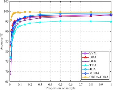
a) All results (Proportion of sample: 0.01-1)
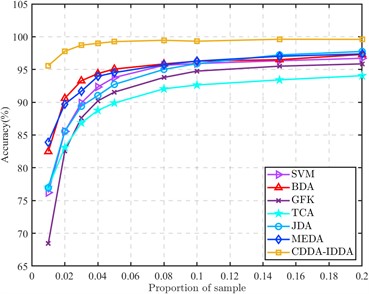
b) Partial results (Proportion of sample: 0.01-0.2)
6.2. Hyperparameter analysis of the overall divergence matrix
In the subspace embedding divergence matrix for divergence alignment, we introduce the regularization parameter . In order to reflect the influence of regularization parameters in the divergence matrix on the diagnostic model, the regularization parameter is analyzed below. The sample ratio of the source domain and the target domain is set to 1:1, and the value is taken at an interval of 0.1 from 0 to 1. Other parameters remain unchanged. Three transfer tasks are selected in the CWRU data set and the composite fault data set for testing, and the experimental results are shown in Fig. 5 and Fig. 6.
It can be seen from the figure that the hyperparameter plays an active role in the different working condition fault identification of rolling bearings. The recognition rate is also gradually improved in the process of gradually increasing the parameters. The accuracy of a single transfer task is improved by 1 % to 8 %, which proves that the introduction of regularization parameters plays a positive role in maintaining the structure of within-class divergence.
6.3. Convergence analysis
In order to study the algorithm convergence of the proposed method, four tasks in the CWRU dataset (F0→F1, F0→F3, F1→F0 and F2→F0) and all tasks in the composite fault dataset are selected for algorithm convergence analysis. The results are shown in Figs. 7 and 8.
Fig. 5Effect of regularization parameter θ on CWRU transfer task
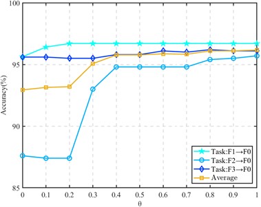
Fig. 6Effect of regularization parameter θ on compound fault transfer task
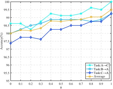
Fig. 7Iteration process (CWRU data)
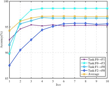
Fig. 8Iteration process (Composite fault data)
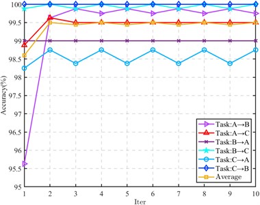
For the transfer task of CWRU data set, the iteration is fast, and it tends to converge after 3 to 5 iterations. In the composite fault data, some tasks obtain better recognition performance in the first iteration. In the subsequent iteration, the recognition rate only fluctuates within a small range, and there is no decrease in the recognition rate. The remaining tasks also tend to be stable after 2 to 3 iterations, indicating that the proposed method has good convergence.
6.4. Ablation analysis
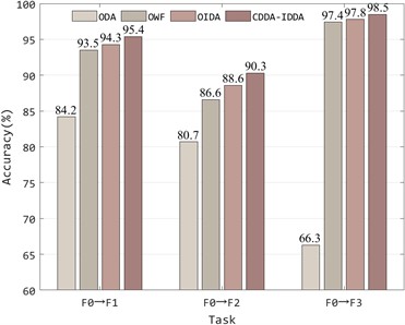
Ablation research is the process of removing some parts of the model to better understand the behavior of the model. In order to deeply analyze the contribution of divergence alignment, cross-domain weighted conditional distribution alignment and inter-class distribution alienation in this method, the first three tasks (F0→F1, F0→F2 and F0→F3) of the CWRU dataset are selected for ablation analysis. Three ablation models based on this method are constructed, which are Omits divergence alignment (ODA), omits weighting factor (OWF) and omits inter-class distribution alienation (OIDA), and compared with this method to obtain the results shown in Fig. 9.
It can be seen from the figure that each part of the fault diagnosis model proposed in this paper plays a positive role in the whole model. Among them, divergence alignment contributes the most to the whole model, and the recognition accuracy is increased by 30 % at most. The accuracy of the transfer task is also slightly improved by the weighting factor and the inter-class distribution alienation term, which proves that each part of the method is indispensable.
Fig. 9Ablation study results
7. Conclusions
In this paper, a rolling bearing fault diagnosis method based on cross-domain divergence alignment and intra-domain distribution alienation (CDDA-IDDA) is proposed, which makes up for the existing domain adaptive methods that only perform cross-domain distribution alignment, or only consider the distribution relationship between classes in the domain, ignoring the inter-domain tilt, failing to take into account these aspects at the same time. In this paper, the existing problems of the current algorithm are corrected by three parts: cross-domain divergence alignment, weighted conditional distribution alignment and inter-class weighted distribution alienation through subspace embedding intra-domain divergence. The experimental results show that the proposed method not only has a good recognition ability for multiple fault types, multiple fault sizes and composite faults, but also maintains the accuracy of the diagnosis model above 95 % when the label samples are scarce.
References
-
N. Huang, X. Yang, and G. Cai, “In-depth confrontation diagnosis of wind turbine main bearing faults using unbalanced small sample data,” Chinese Journal of Electrical Engineering, Vol. 40, No. 2, pp. 563–574, 2020.
-
D. Wang, “K-nearest neighbors based methods for identification of different gear crack levels under different motor speeds and loads: Revisited,” Mechanical Systems and Signal Processing, Vol. 70-71, pp. 201–208, Mar. 2016, https://doi.org/10.1016/j.ymssp.2015.10.007
-
Q. Shi, X. Guo, and D. Liu, “Bearing fault diagnosis based on feature fusion and support vector machine,” Journal of Electronic Measurement and Instrumentation, Vol. 33, No. 10, pp. 104–111, 2019.
-
Y. Zhang, Chen Jun, and X. Wang, “Application of random forest in fault diagnosis of rolling bearings,” Computer Engineering and Applications, Vol. 54, No. 6, pp. 100–104, 2018.
-
F. Zhuang, P. Luo, and Q. He, “Research progress of transfer learning,” Journal of Software, Vol. 26, No. 1, pp. 26–39, 2015.
-
E. Inoue, M. Rabbani, and M. Mitsuoka, “Investigation of nonlinear vibration characteristics of agricultural rubber crawler vehicles,” AMA-Agricultural Mechanization in Asia Africa and Latin America, Vol. 40, No. 1, pp. 89–93, 2014.
-
B. Shen, B. Chen, and C. Zhao, “Research review of deep learning in failure prediction and health management of mechanical equipment,” Machine Tool and Hydraulics, Vol. 49, No. 19, pp. 162–171, 2021.
-
H. Wang, L. Geng, and T. Ni, “Transfer twin support vector machine for knowledge embedding,” Control and Decision, Vol. 34, No. 3, pp. 519–526, 2019.
-
H. Zhang, X. Han, and K. Shi, “Research on online diagnosis system of hoist spindle fault based on deep transfer learning,” Coal Engineering, Vol. 54, No. 7, pp. 61–66, 2022.
-
R. Chen, L. Tang, and X. Hu, “Fault diagnosis method of rolling bearing based on deep attention transfer learning at different rotational speeds,” Vibration and Shock, Vol. 41, No. 12, pp. 95–101, 2022.
-
H. Xu, W. Zhang, D. Song, and B. Chen, “Research on fault diagnosis method of SSDAE rolling bearing based on deep migration,” Noise and Vibration Control, Vol. 41, No. 6, pp. 112–118, 2021.
-
Y. Lan, C. Hu, J. Jin, and Y. Wang, “Research on cross-domain bearing fault classification method based on migration component analysis,” Mechanical and Electrical Engineering, Vol. 38, No. 5, pp. 521–527, 2021.
-
R. Chen, S. Chen, and X. Hu, “Recognition of rolling bearing life state under different working conditions with multi-sample integrated GFK in source domain,” Chinese Journal of Vibration Engineering, Vol. 33, No. 3, pp. 614–621, 2020.
-
J. Wang, W. Feng, and Y. Chen, “Visual domain adaptation with manifold embedded distribution alignment,” in ACM Multimedia Conference in Seoul, pp. 402–410, 2018.
-
M. Long, J. Wang, and G. Ding, “Transfer feature learning with joint distribution adaptation,” in IEEE International Conference on Computer Vision, pp. 2200–2207, 2013.
-
X. Zhang, D. Yu, and S. Liu, “Research on small sample bearing fault diagnosis method based on transfer learning,” Journal of Xi’an Jiaotong University, Vol. 55, No. 10, pp. 30–37, 2021.
-
K. Zhao, H. Jiang, Z. Wu, and T. Lu, “A novel transfer learning fault diagnosis method based on Manifold Embedded Distribution Alignment with a little labeled data,” Journal of Intelligent Manufacturing, Vol. 33, No. 1, pp. 151–165, Jan. 2022, https://doi.org/10.1007/s10845-020-01657-z
-
J. Gao, R. Huang, and H. Li, “Sub-domain adaptation learning methodology,” Information Sciences, Vol. 298, No. 20, pp. 237–256, Mar. 2015, https://doi.org/10.1016/j.ins.2014.11.041
-
B. Fernando, A. Habrard, M. Sebban, and T. Tuytelaars, “Unsupervised visual domain adaptation using subspace alignment.,” in IEEE International Conference on Computer Vision, pp. 2960–2967, 2013.
-
Z. Zheng, C. Hu, and X. Jiang, “Deep transfer adaptation network based on improved maximum mean difference algorithm,” Computer Applications, Vol. 40, No. 11, pp. 3107–3112, 2020.
-
J. Wang, Y. Chen, and S. Hao, “Balanced distribution adaptation for transfer learning,” in IEEE International Conference on Data Mining, pp. 129–1134, 2017.
-
Belkinmikhail, Niyogipartha, and Sindhwanivikas, “Manifold regularization: A geometric framework for learning from labeled and unlabeled examples,” The Journal of Machine Learning Research, Vol. 7, pp. 2399–2434, Dec. 2006, https://doi.org/10.5555/1248547.1248632
-
B. Gong, Y. Shi, and F. Sha, “Geodesic flow kernel for unsupervised domain adaptation,” in 25TH IEEE Conference on Computer Vision and Pattern Recognition, pp. 2066–2073, 2012.
-
S. J. Pan, I. W. Tsang, J. T. Kwok, and Q. Yang, “Domain adaptation via transfer component analysis,” IEEE Transactions on Neural Networks, Vol. 22, No. 2, pp. 199–210, Feb. 2011, https://doi.org/10.1109/tnn.2010.2091281
About this article

Financial support from Guangdong Basic and Applied Basic Research Fund Enterprise Joint Fund (Offshore Wind Power) Project (Grant No. 2022A515240043), Guangdong Natural Science Foundation Project (Grant No. 2023A1515012698) and the Special Research Project on the Key Fields in General Universities of Guangdong Province (Grant No. 2020ZDZX2033) is appreciated.
The datasets generated during and/or analyzed during the current study are available from the corresponding author on reasonable request.
Shubiao Zhao: conceptualization, data curation, methodology, software, validation, visualization, writing – original draft preparation. Guangbin Wang: conceptualization, formal analysis, funding acquisition, investigation, project administration, resources, writing-review and editing. Xuejun Li: funding acquisition, project administration, supervision. Junhua Chen: conceptualization, writing-original draft preparation. Lingli Jiang: formal analysis, project administration.
The authors declare that they have no conflict of interest.
