Abstract
In the power line communication network, the electrical node switch connected to the Power Line Communication network will affect the impedance, noise and signal attenuation of the network. The connection change between the network nodes will lead to the change of the topology structure. This paper proposes a new type of automatic modulation pattern recognition system assisted by blind channel recognition based on a convolutional neural network, which is composed of two convolutional neural networks with different architectures, and successfully improves the recognition accuracy of the traditional automatic modulation pattern recognition system. The Signal to Noise Ratio recognition rate of the proposed blind channel recognition assisted Adaptive Multi-Rate system is as high as 99 %, which is more than 5 % higher than that of other comparison methods. After several iterations, the accuracy and loss function of the model studied in this paper are still at a stable level. The intelligent recognition technology of blind signals proposed in this paper can effectively improve the interference problem of communication signals in power system and has a promotion effect in other communication systems, which can achieve higher technical application value.
Highlights
- Classifying wireless communication signals by a deep learning algorithm
- Optimizing the parameters and depth of the convolutional neural network to achieve better recognition performance
- Enhancing the stability and reliability of the power line communication network by using the route reconstruction strategy which combines the direct route reconstruction mode and the indirect route reconstruction mode
1. Introduction
With the development and integration of power industry technology and Internet of Things technology, a new network form of power Internet of Things has been formed. Power Internet of Things applies Internet of things technology to smart grid, integrates infrastructure resources of communication and power system, and effectively improves the utilization efficiency of the existing infrastructure of the power system. It is used to realize the collection of information flow in power generation, transmission, transformation, distribution, and utilization of power systems [1]. The technical architecture of the power Internet of Things mainly includes the application layer, the network layer, and the perception layer. The perception layer is the underlying foundation of the physical form of the power Internet of Things. It mainly uses technologies such as intelligent sensing and intelligent chips of terminal equipment to realize the collection, processing, control, and interaction of information in power production, transmission, and consumption management. In the aspect of the network layer, the equipment is mainly connected to the network by means of power wireless private network, power optical fiber private network and power line carrier communication network [2]. The information perception technology and communication access of the Internet of Things involved in the perception layer and the network layer are the basis and premise for realizing the effective work of the application layer of the Internet of Things [3].
The topological structure of the distribution grid is relatively complex, and it is difficult to meet the needs of all power Internet of Things information sensing terminals in various environments only by power line communication [4]. The use of multiple communication mode integration technology can improve the coverage of the overall communication network and ensure the data transmission needs of the power Internet of Things sensing layer and application layer [5]. Wireless communication technology has the advantage of flexible access. PLC (Power Line Communication) communication technology is easily affected by line load and interference [6]. The integration of wireless communication technology and power line communication technology, giving full play to their respective technical advantages, is conducive to improving the communication reliability of the power Internet of Things information perception system [7]. Therefore, it is of great academic significance and engineering application value to study the key technologies of power lines and wireless communication convergence [8].
In reference [9], based on the theory of multi-conductor transmission line, the channel model of a three-core power line in the frequency range from 30 kHz to 15 MHz is proposed. The channel model has high accuracy and considers the influence of network structure on impedance and transmission characteristics. In reference [10], the power line MIMO (Multiple-Input Multiple-Output) channel model is modified to a multipath model in the presence of impulse noise and background noise. The link-level performance of a medium-voltage MIMO-OFDM communication system based on an underground power line channel transmission link is evaluated [11]. The effects of three impedance matching criteria on receiver SNR and system capacity are studied, and a simplified impedance matching criterion is proposed. Reference [12] analyzes the simplified distributed parameter model of the power line and calculates the impedance of the power line. A low-cost and compact band-pass matching coupler is designed, which can match the impedance on the basis of accurately calculating the impedance of the power lines. Document [13] designs a T-shaped adaptive impedance matching system based on the T-shaped network complex impedance matching method of resonance and absorption. By adjusting the component values of the T-shaped network, the adaptive impedance matching between the vehicle power line communication modem and the vehicle power line network is realized. Reference [14] designed an impedance-adaptive bidirectional transformer coupling circuit for the low-voltage power line communication. The coupling transformer can equalize the terminal impedance on either side to achieve maximum power transmission. Reference [15] measured impulse noise from power line networks in three different environments and performed multifractal analysis. The power line noise exhibits both long-range correlation and multifractal scaling behavior with different intensities. Reference [16] proposes an adaptive impulse noise mitigation system based on time-varying impulse noise channel. According to the method of torque estimation to pre-evaluate the impulse noise characteristics, an adaptive iterative impulse noise mitigation module is designed, which can achieve performance balance in different degrees of impulse noise environment. Power line communication technology can make full use of the existing physical network of the power distribution network for communication and data transmission, with the characteristics of small investment, strong flexibility and wide coverage, but due to the serious electromagnetic interference of the power distribution network, large channel attenuation and other factors. As a result, the communication quality is relatively poor [17]. To solve the problems of coverage and reliability of power line communication network in distribution power grid, a networking method suitable for power line communication is studied, and the automatic networking and dynamic maintenance of the network are realized by designing the corresponding power line communication protocol, networking process and routing reconstruction strategy. It is of great significance to improve the reliability of power line communication network.
Therefore, the automatic modulation pattern recognition technology based on BP neural network proposed in this paper mainly uses the model of a deep convolutional neural network to realize the pattern recognition of unknown wireless modulation signals. The simulation results show that the recognition accuracy of the AMR (Adaptive Multi-Rate) system based on the deep convolutional neural network proposed in this paper is obviously better than that of the traditional AMR recognition method.
The main innovations of this paper are:
– A deep learning algorithm is used to classify wireless communication signals. The selected two types of signals are mainly modulation signals and LTE-U and Wi-Fi signals in unlicensed frequency bands.
– Optimize the parameters and depth of the convolutional neural network to achieve better recognition performance.
– The stability and reliability of the power line communication network are enhanced by using the route reconstruction strategy which combines the direct route reconstruction mode and the indirect route reconstruction mode.
2. Related researches
2.1. Communication signal identification
Due to the increasingly complex wireless communication environment, the transmission space of electromagnetic signals is becoming more and more complex. When the amount of information transmitted becomes larger, the change of signals will also become faster [18]. Therefore, in the current environment, there is an urgent need to develop a method and a device for modulating a signal using different modulation modes, such as Frequency Shift Keying (FSK), Quadrature Amplitude Modulation (QAM), Efficient Automatic Modulation Recognition (AMR) method [19] for wireless signals under QAM, etc.
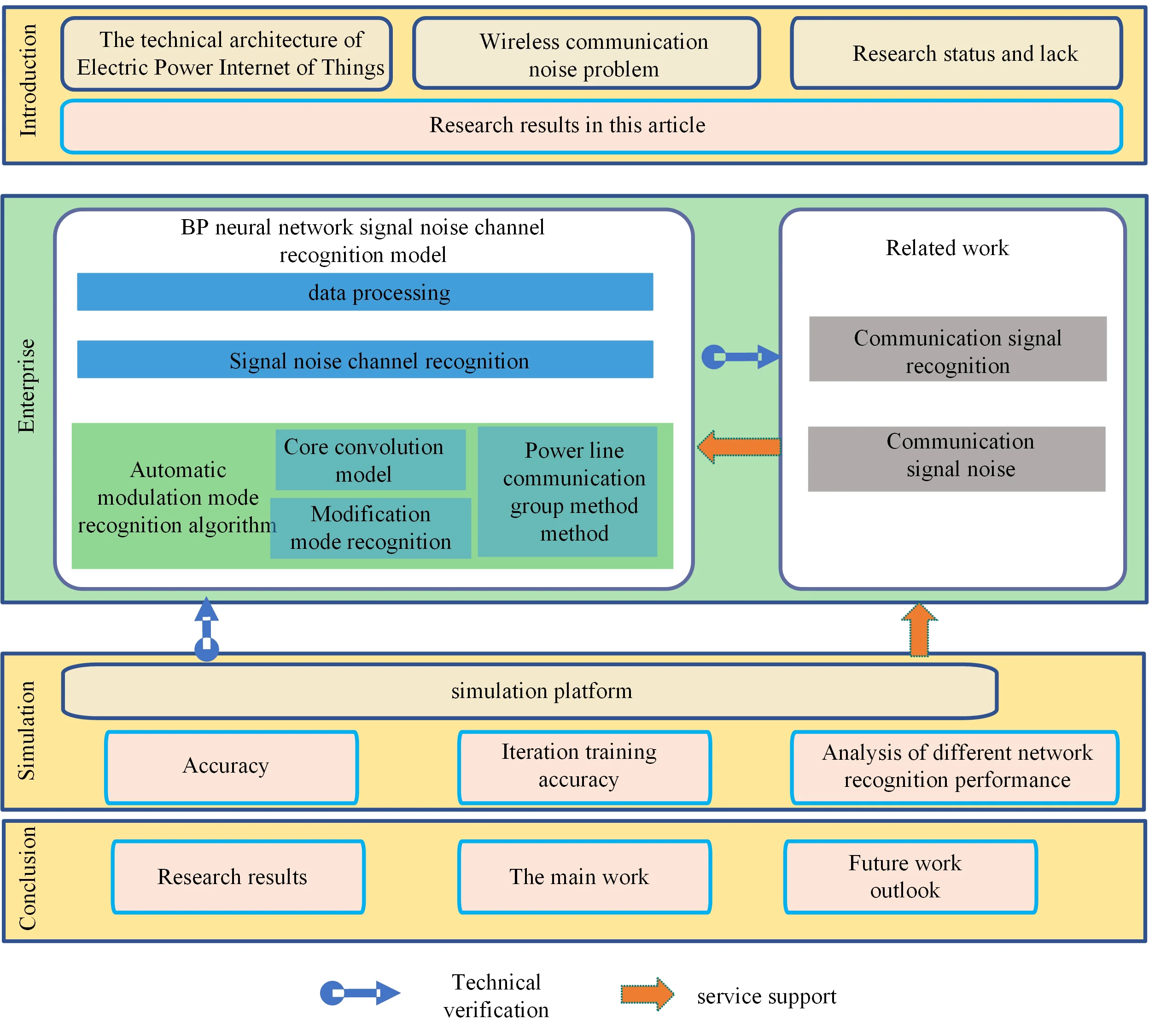
The statistics-based pattern recognition system can be divided into two subsystems: Feature Extraction and Pattern Classification. The function of the first subsystem feature extraction is to extract the feature parameters defined in the received modulated wireless signal and reduce the dimensionality of the pattern representation, such as instantaneous features, Fourier transform, wavelet transform, higher order cumulants (HOC), etc. [20]. The second subsystem, pattern classification, can use algorithms such as Artificial Neural Networks (ANN), Support Vector Machines (SVM), and decision trees to identify the modulation patterns of wireless signals. The signal recognition pattern structure is shown in Fig. 1.
Fig. 1Basic architecture of pattern recognition system
With the increasing popularity of artificial intelligence technology, deep learning algorithms have been widely used in physical layer applications of wireless communications. Researchers have used deep learning algorithms to build neural network models, thus proposing many methods to achieve better classification performance. Some scholars proposed to train AMR (Automatic Modulation Recognition) system based on the algorithm model of deep convolutional neural network to achieve high-precision modulation pattern recognition [21].
2.2. Communication signal noise
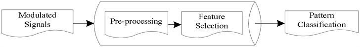
Compared with traditional methods, the two AMR algorithms based on deep learning can achieve higher pattern recognition accuracy and perform well. When the signal passes through the line-of-sight channel. The modulated signal is connected to the AMR system that has been trained for the line-of-sight channel to achieve high-precision identification [22], which is shown in Fig. 2.
In this paper, taking channel conditions only including LOS and non-LOS as an example, Fig. 2(a) is the identification confusion matrix of six modulation mode signals when wireless modulation signals under LOS channel conditions are accessed to the AMR system trained for the LOS channel. Fig. 2(b) is an identification confusion matrix for six modulation modes in an AMR system with a non-line-of-sight (NLOS) channel training number accessed by a wireless modulation signal under the NLOS channel condition. From the confusion matrix, it can be seen that when the wireless modulation signal is accessed to the corresponding AMR system, the recognition accuracy is very high, reaching more than 95 %. The color of the square on the diagonal of each modulation mode is very dark, indicating that the system has accurately identified the six modulation signals.
Fig. 2Confusion matrix in AMR system with matched input signal channel condition
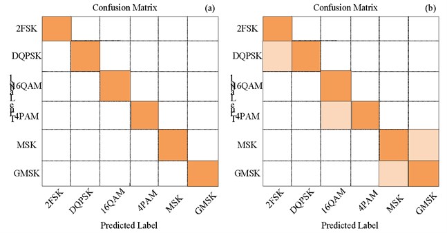
In the actual situation, when the input wireless modulation signal does not meet the preconditions, for example, when the wireless modulation signal passes through the line-of-sight channel, the signal is connected to the AMR system trained as a non-line-of-sight channel. The recognition effect will certainly deteriorate [23], which is shown in Fig. 3.
Fig. 3Confusion matrix of AMR system with mismatched input signal channel condition
This paper shows the performance of AMR systems when the channel conditions do not correspond. Fig. 3(a) is an identification confusion matrix of signals of six modulation modes when a wireless modulation signal under the condition of a line-of-sight channel is accessed to an AMR system trained for a non-line-of-sight channel. Fig. 3(b) is an identification confusion matrix of signals of six modulation modes when a wireless modulation signal under the condition of a non-line of sight channel is accessed to an AMR system trained for a line-of-sight signal. The average recognition accuracy of Fig. 3(a) is 80 %, and the channel performs poorly in recognizing MSK and GMSK modulation signals. The average recognition accuracy of Fig. 3(b) is only 50 %, and the modulation mode of the signal can hardly be recognized.
3. Identification model of signal and noise channels based on BP neural network
3.1. Data processing
To test the proposed algorithm, two separate data sets are created, which are the training set and the test set. This paper assumes that the selected channel conditions are line-of-sight and non-line-of-sight channels, and each data set contains modulated signal data passing through the two channel conditions. Six modulation modes are selected for the modulation signals under each channel condition, namely, binary frequency shift keying (2FSK), quadrature phase shift keying (DQPSK), quadrature amplitude modulation (16Qam), quadrature-phase pulse amplitude modulation (4Pam), minimum frequency shift keying (MSK) and Gaussian minimum frequency shift key (GMSK). The number of signal samples in each modulation mode is 2000, and the ratio of the training set to the test set is 1:1, so there are 24,000 samples in each data set. First, perform in-phase and quadrature sampling on randomly input modulated signals passing through line-of-sight and non-line-of-sight channels. The sampling length is 256, so the data matrix of each sampled signal is . Each signal is also sampled to mark the channel conditions through which it passes. Then, the additive white Gaussian noise is introduced to the IQ data of all signals, so that each modulated signal has a different degree of Signal-to-Noise Ratio (SNR). Ultimately, the signal-to-noise ratio of the signal for each data set ranges from 0 to 12 dB with a 2 dB separation, i.e. . The seven data sets with different SNR will be sent to the AMR system of signal and noise channel recognition based on the BP neural network proposed in this paper to compare the influence of SNR on the recognition effect.
3.2. Signal and noise channel identification
In this paper, a new automatic modulation mode identification algorithm assisted by Signal noise channel identification (SNCI) based on BP neural network is proposed, and the system model box of the algorithm is shown in Fig. 4.
Fig. 4AMR system model aided by signal and noise channel identification
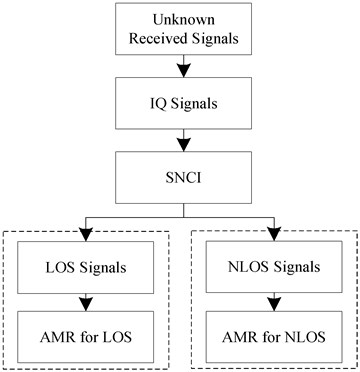
In this AMR system, the core goal is to accurately classify the modulation pattern of the unknown signal. In Fig. 4, the system input is an unknown wireless modulation mode signal and the whole system is composed of two deep convolutional neural models. After the arrival of Unknown Received Signals, they are preprocessed first, and their in-phase and quadrature characteristics are extracted to form IQ data. The modulation signals extracted as in-phase and quadrature features are then sent to the first trained deep convolutional neural network for signal and noise channel identification to distinguish whether the modulation signal passes through the line-of-sight channel or the non-line-of-sight channel. Finally, after identifying the channel conditions of the modulated signal, the modulated signal is fed into a second deep convolutional neural model: a common AMR system trained in advance to match the modulated signal. A completely unknown modulation signal can be accurately identified by the proposed AMR system assisted by blind signal identification based on neural network.
4. Automatic modulation pattern recognition algorithm
4.1. Core convolution model
It can be known from the system model that the modulated signal is extracted as in-phase and quadrature characteristic data and then sent to the first trained deep convolutional neural model for signal and noise channel identification to distinguish whether the modulated signal passes through a line-of-sight channel or a non-line-of-sight channel. Signal and noise channel identification using the first deep convolutional neural. After each neural network layer, a batch normalization (BN) layer and an activation function layer are added. The function of the batch standardization layer is to select a larger learning rate to achieve a faster training speed for the model and make the neural network model converge quickly. Since each layer of the network causes a change in the data distribution, preprocessing at the input layer is required.
Specify that the output of the input data through one layer of batch normalization is:
Then the data after one layer of batch standardization is sent to the next layer of deep convolutional nerve as the input of the next layer. The data that each network layer needs to learn and extract has been standardized in batches in the previous network layer, and the features obtained must deviate from the initial data. Batch normalization affects the features learned and extracted from the previous network layer. Some improvements need to be made to the above method, and the output data of each layer needs to be transformed, reconstructed and introduced into the parameters that can be learned:
Through such formula conversion, it can effectively prevent the hidden features in the data from deviating too much from the initial data after the batch standardization of each layer, and enhance the expression ability of each neural network layer. In addition, and are defined as follows:
By introducing parameters that can be learned, the trained neural network can recover the distribution of hidden features in the original data, and can recover the features learned and extracted from the original layer data in each neural network layer to enhance the network expression ability. Finally, the activation function layer uses the “Parametric Rectified Linear Unit” function, which is distributed after each convolution layer and the fully connected layer.
4.2. Modulation pattern recognition
After the first deep convolutional neural model identifies the channel condition of the unknown modulation signal, the second deep convolutional neural model is used to accurately identify the six modulation mode signals under the specified channel condition. Therefore, it is necessary to train the AMR model under the condition of line-of-sight and non-line-of-sight channels respectively. Table 1 shows the model structure of the deep convolutional neural.
Table 1Deep convolutional neural parameters for modulation pattern recognition
Layer | Output dimensions |
Input | 2×256×1 |
Conc2D (filters 128, size 1×8) + PReLU | 2×249×128 |
Dropout (0.6) | – |
Conc2D (filters 64, size 1×4) + PReLU | 2×249×64 |
Dropout (0.6) | – |
Flatten | 31488 |
Dense + PReLU | 256 |
Dropout (0.6) | – |
Dense + PReLU | 128 |
Dropout (0.6) | – |
Dense + SoftMax | Modulation modes |
In Table 1, it consists of two parts, two convolutional layers and three fully connected layers. The first convolution layer consists of 128 convolution kernels, each of size 1×8. Secondly, the second convolution layer contains 64 convolution kernels, and the convolution kernel size is 1×4. The convolutional layer is followed by three fully connected layers. Based on the strategy that every neuron in the former fully connected layer is connected to all neurons in the latter fully connected layer, the number of neurons in the first and second fully connected layers is 256 and 128, respectively. The third fully connected layer, also known as the output layer, can obtain the output of the entire network. The number of neurons it has is the number of modulation modes used by the signal to be identified. There are six modulation modes involved in this paper.
In addition, an activation function layer and a Dropout layer are added after each convolutional network layer and the fully connected layer. The activation function used is still the PReLU function to prevent overfitting problems. The parameter value of the dropout layer is set to 0.6, that is, nearly 60 % of the neurons are ignored in the training process. Finally, Softmax is used as the activation function of the output layer, which can directly calculate the probability of the possible modulation mode of the test signal according to all the extracted features and the parameters trained by the classification layer, and select the class with the highest probability as the prediction result of the whole deep convolutional neural model.
4.3. Power line communication networking method
In the process of building the power line communication network, the actual situation is more complex. For the convenience of discussion, the research in this section is based on the following assumptions: any two nodes can communicate in both directions in principle, that is, the power line communication link is a symmetrical link. There is no communication blind spot in the power line communication network, that is, any node can communicate with the central node in principle. Each node can calculate the communication rate, delay and packet loss rate data between it and the previous node after receiving the networking packet, and store them in the QoS parameter routing table.
This paper refers to the DL/T645-2007 and IEC870-5-101 communication protocol. Combined with the requirements of the I-LDAQ algorithm of power line communication quality of service constraints, the corresponding communication protocol is designed. The standard data frame format is shown in Fig. 5.
It can be seen from Fig. 5 that in the frame format, the frame start symbol and the frame end symbol respectively represent the start and the end of the data frame. The control code is used to control different data frame functions. The source node and the destination node respectively represent the network numbers of the data sending node and the data receiving node. The relay node represents the network number of the relay route through which the data packet passes from the source node to the destination node. The data length field and the data field are used to represent the relevant information of the transmitted data. The check code is responsible for checking the data of all bytes from the frame start character to the data field.
Fig. 5Standard data frame format

If there are k points that can directly communicate with the node, the routing table needs to record the QoS data of the group, that is, the delay, packet loss rate, and communication rate on path . The QoS parameter routing table of the node is shown in Table 2.
To make the network packets select the next hop routing according to the state transition probability, each communication node needs to store the pheromone table, including the group pheromone and the group pheromone.
Table 2QoS parameter routing table
Routing node number | Delay | Packet loss rate | Communication rate |
… | … | … | … |
= {0 dB, 2 dB, 4 dB, 6 dB, 8 dB, 10 dB} |
5. Simulation experiment analysis
5.1. Simulation platform
After preprocessing the signal samples, the processed signals can be connected to the neural network algorithm model for training. The deep learning algorithms used in the complex heterogeneous network intelligent signal recognition technology include fully connected deep neural network (FC-DNN), convolutional neural network (CNN), and recurrent neural network (RNN). The parameter value of the dropout layer is set to 0.5, that is, close to 50 % of the neurons are ignored in the training process. The third fully connected layer (which is also used as the output layer of the convolutional neural network structure) contains two neurons, and the number of neurons in this layer is directly linked to the type of signal we want to identify. Generally, the activation function of the output layer uses the Softmax function, which can directly calculate the probability of whether the test signal belongs to LTE or WiFi signal according to all the extracted features and the parameters trained by the classification layer, and select the one with the highest probability as the prediction result of the whole convolutional neural network.
The training, validation and testing of all the deep learning algorithm models used in this experiment are based on the Python 3.7 computer language using the Keras software library version 2.2.2. The experimental platform configuration is shown in Table 3.
Table 3Experimental platform configuration
Settings | Parameters |
CPU | Intel I7-10750H 5.0 GHz |
Memory | 32GDDR4 |
Hardware | 1T SSD |
System | Windows 10 |
5.2. Experimental analysis
5.2.1. Recognition accuracy
The first trained deep convolutional neural network is used to identify the channel conditions through which the unknown modulated signal after IQ sampling passes during transmission. The signal-to-noise ratio range of the data set sent to the deep convolutional neural network is {0 dB, 2 dB, 4 dB, 6 dB, 8 dB, 10 dB}. Five deep learning or machine learning algorithms were used to train and test, and their automatic modulation pattern recognition accuracy was compared. They are deep convolutional neural network (CNN), deep convolutional neural network without batch normalization layer, recurrent neural network, BP neural network (DNN) with high-order cumulant (HOC) extraction features, and random forest (RF) classification algorithm with high-order cumulant extraction features. The computer simulation results of signal and noise channel identification are shown in Fig. 6.
Fig. 6Recognition accuracy of five algorithms under different SNR conditions
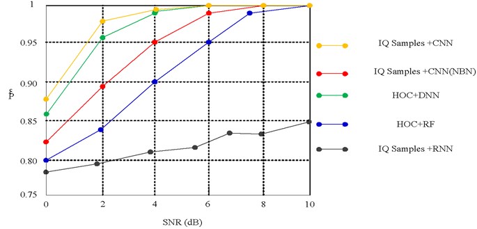
With the improvement of the signal-to-noise ratio, the recognition performance of each algorithm in the figure has been significantly improved. In particular, the recognition accuracy of the deep convolutional neural algorithm is very high. The probability of correctly recognizing the channel condition can reach more than 99 % under the condition of high signal-to-noise ratio. And no matter what kind of SNR conditions, the recognition effect of deep convolution neural algorithm model is better than other algorithms. In contrast, the recognition effect of the BP neural network algorithm and the random forest algorithm is slightly inferior. In addition, it can be noted that the recurrent neural network algorithm model does not achieve good performance, and the classification accuracy is not very high. This may be because the wireless signal is too random and has no temporal correlation when it passes through certain channel conditions, so the continuous input of signal samples can not improve the accuracy of recurrent neural network.
5.2.2. Iterative training accuracy
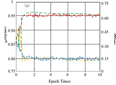
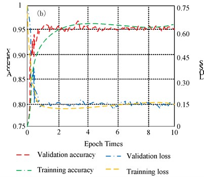
Through the previous comparison of recognition accuracy, we can see that whether the deep convolutional neural algorithm model contains the batch normalization layer has little difference in the recognition results, and they are all excellent. To visualize the impact of adding a batch normalization layer after each network layer on the algorithm model. The training and validation curves of the complete deep convolutional neural network with or without the batch normalization layer training process are plotted in Fig. 7.
In Fig. 7, the abscissa represents the training times, the left ordinate represents the accuracy rate, and the right ordinate represents the loss function value. Comparing the curves of the two figures, it can be clearly seen that due to the lack of batch normalization layer, the curves of the accuracy and loss function values of the deep convolutional neural model will fluctuate sharply, which is difficult to stabilize and takes a long time to converge. However, after adding the batch normalization layer, the curves of the accuracy and loss function values of the deep convolutional neural model will converge quickly and smoothly, and eventually, the training and verification curves will be basically similar.
Fig. 7Deep convolutional neural training and validation curves
5.2.3. Performance analysis of different network identification
Because the other two algorithms can not identify the signal, only two curves of the CNN model are observed. The evaluation results are shown in Fig. 8.
Fig. 8Recognition accuracy of deep learning algorithm under different conditions
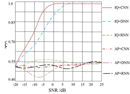
When SNR is higher than 5 dB, that is, under the condition of high signal-to-noise ratio, the curves of IQ data form and AP data form are almost coincident, and the accuracy is very high. It can be seen that in the case of good channel conditions, the results of the two data modes are not very different. However, notice the difference in SNR between –10 dB and 0 dB, and the effect of using IQ as the input data is better than that of using AP as the input data. When SNR = –5 dB, the difference between them is the most obvious, the recognition accuracy of IQ data is 96 %, while the recognition accuracy of AP data is only 67 %, and the difference between them is close to 30 %. This indicates that the input data in the form of IQ is better able to effectively distinguish between LTE-U and WiFi signals under low SNR conditions.
6. Conclusions
In this paper, the deep learning algorithm is combined with the classification of wireless communication signals. The two directions of modulation signal identification and interference signal identification of wireless communication signal identification are studied. Based on two deep convolutional neural architectures, a novel automatic modulation pattern recognition technology assisted by signal and noise channel recognition is proposed. The recognition performance of Wi-Fi and LTE-U signals in the unlicensed frequency bands is analyzed by using various deep neural network algorithms and models. Finally, it is found that the recognition accuracy of the convolutional neural network is the highest, which can effectively realize the friendly coexistence of LTE-U and Wi-Fi signals. The main work is as follows:
1) The significance of automatic modulation recognition and the problems of existing AMR systems are analyzed.
2) Design a neural architecture with double depth convolution, wherein the AMR system can obtain higher recognition accuracy when recognizing the modulation mode.
3) Simulation results show that the proposed AMR system with the aid of signal and noise channel identification can replace the traditional AMR system in many applications.
In future work, we will focus on the robustness of deep convolutional neural-based classifiers in a large signal-to-noise ratio range and further improve the recognition accuracy in many applications.
References
-
W. Lin, Z. Yang, X. Hong, S. Wang, and J. Wu, “Brillouin gain bandwidth reduction in Brillouin optical time domain analyzers,” Optics Express, Vol. 25, No. 7, p. 7604, Apr. 2017, https://doi.org/10.1364/oe.25.007604
-
B. Wang, D. Ba, Q. Chu, L. Qiu, D. Zhou, and Y. Dong, “High-sensitivity distributed dynamic strain sensing by combining Rayleigh and Brillouin scattering,” Opto-Electronic Advances, Vol. 3, No. 12, pp. 20001301–20001315, 2020, https://doi.org/10.29026/oea.2020.200013
-
J. B. Murray and B. Redding, “Combining Stokes and anti-Stokes interactions to achieve ultra-low noise dynamic Brillouin strain sensing,” APL Photonics, Vol. 5, No. 11, p. 116104, Nov. 2020, https://doi.org/10.1063/5.0024121
-
H. Zheng et al., “Polarization independent fast BOTDA based on pump frequency modulation and cyclic coding,” Optics Express, Vol. 26, No. 14, p. 18270, Jul. 2018, https://doi.org/10.1364/oe.26.018270
-
B. Wang, N. Guo, L. Wang, C. Yu, and C. Lu, “Robust and fast temperature extraction for Brillouin optical time-domain analyzer by using denoising autoencoder-based deep neural networks,” IEEE Sensors Journal, Vol. 20, No. 7, pp. 3614–3620, Apr. 2020, https://doi.org/10.1109/jsen.2019.2960876
-
H. Zheng, J. Zhang, H. Wu, N. Guo, and T. Zhu, “Single shot OCC-BOTDA based on polarization diversity and image denoising,” Optics and Lasers in Engineering, Vol. 137, p. 106368, Feb. 2021, https://doi.org/10.1016/j.optlaseng.2020.106368
-
N. Srinivas, G. Pradhan, and P. K. Kumar, “A classification-based non-local means adaptive filtering for speech enhancement and its FPGA prototype,” Circuits, Systems, and Signal Processing, Vol. 39, No. 5, pp. 2489–2506, May 2020, https://doi.org/10.1007/s00034-019-01267-y
-
Z. Fang and X. Yi, “A novel natural image noise level estimation based on flat patches and local statistics,” Multimedia Tools and Applications, Vol. 78, No. 13, pp. 17337–17358, Jul. 2019, https://doi.org/10.1007/s11042-018-7137-4
-
Z. Zhao, C. Yao, C. Li, and S. Islam, “Detection of power transformer winding deformation using improved FRA based on binary morphology and extreme point variation,” IEEE Transactions on Industrial Electronics, Vol. 65, No. 4, pp. 3509–3519, Apr. 2018, https://doi.org/10.1109/tie.2017.2752135
-
S. Huang et al., “Automatic modulation classification using gated recurrent residual network,” IEEE Internet of Things Journal, Vol. 7, No. 8, pp. 7795–7807, Aug. 2020, https://doi.org/10.1109/jiot.2020.2991052
-
F. Meng, P. Chen, L. Wu, and X. Wang, “Automatic modulation classification: a deep learning enabled approach,” IEEE Transactions on Vehicular Technology, Vol. 67, No. 11, pp. 10760–10772, Nov. 2018, https://doi.org/10.1109/tvt.2018.2868698
-
J. Zheng and Y. Lv, “Likelihood-based automatic modulation classification in OFDM with index modulation,” IEEE Transactions on Vehicular Technology, Vol. 67, No. 9, pp. 8192–8204, Sep. 2018, https://doi.org/10.1109/tvt.2018.2839735
-
B. Wang et al., “Spatial-wideband effect in massive MIMO with application in mmWave systems,” IEEE Communications Magazine, Vol. 56, No. 12, pp. 134–141, Dec. 2018, https://doi.org/10.1109/mcom.2018.1701051
-
B. Tang, Y. Tu, Z. Zhang, and Y. Lin, “Digital signal modulation classification with data augmentation using generative adversarial nets in cognitive radio networks,” IEEE Access, Vol. 6, pp. 15713–15722, 2018, https://doi.org/10.1109/access.2018.2815741
-
S. Santra, A. Lahiri, and N. C. Das, “Dynamic problem in 3D thermoelastic half-space with rotation in context of G-N type II and type III,” Mathematical Models in Engineering, Vol. 3, No. 1, pp. 58–70, Jun. 2017, https://doi.org/10.21595/mme.2017.18143
-
P. Bałazy, P. Gut, and P. Knap, “Convolutional mask-wearing recognition algorithm for an interactive smart biometric platform,” Robotic Systems and Applications, Vol. 1, No. 2, pp. 35–40, Sep. 2021, https://doi.org/10.21595/rsa.2021.22108
-
J. Liu, C. Zhang, G. Liu, S. Chu, S. Li, and J. Zhang, “Study on swage autofrettage of steel sleeve for the high pressure plunger pump,” Journal of Measurements in Engineering, Vol. 9, No. 3, pp. 128–141, Sep. 2021, https://doi.org/10.21595/jme.2021.21962
-
G. Shuqing and S. Yucong, “Traffic sign recognition based on HOG feature extraction,” Journal of Measurements in Engineering, Vol. 9, No. 3, pp. 142–155, Sep. 2021, https://doi.org/10.21595/jme.2021.22022
-
G. Shuqing and L. Yuming, “Traffic signal light detection and recognition based on canny operator,” Journal of Measurements in Engineering, Vol. 9, No. 3, pp. 167–180, Sep. 2021, https://doi.org/10.21595/jme.2021.22024
-
Y. S. K. Osman and E. I. Salim, “A fuzzy logic monitoring system (FLMS) based on visible light and EMF effects on experimental animals,” Journal of Mechatronics and Artificial Intelligence in Engineering, Vol. 2, No. 1, pp. 30–43, May 2021, https://doi.org/10.21595/jmai.2021.21879
-
Y.-D. Xu, “Effect of cutting angle on the performance of the head of a roadheader,” Journal of Mechatronics and Artificial Intelligence in Engineering, Vol. 2, No. 1, pp. 54–62, Jun. 2021, https://doi.org/10.21595/jmai.2021.22042
-
P. T. Lin, Z.-Y. Chen, P.-R. Liaw, and V. L. Nguyen, “Design of a high-payload Mecanum-wheel ground vehicle (MWGV),” Robotic Systems and Applications, Vol. 1, No. 1, pp. 24–34, Jun. 2021, https://doi.org/10.21595/rsa.2021.22133
-
A. Idzkowski and Z. Warsza, “Temperature difference measurement with using two RTD sensors as example of evaluating uncertainty of a vector output quantity,” Robotic Systems and Applications, Vol. 1, No. 2, pp. 53–58, Nov. 2021, https://doi.org/10.21595/rsa.2021.22143
About this article

