Abstract
There is an ever-increasing need to optimise bearing lifetime and maintenance cost through detecting faults at earlier stages. This can be achieved through improving diagnosis and prognosis of bearing faults to better determine bearing remaining useful life (RUL). Until now there has been limited research into the prognosis of bearing life in rotating machines. Towards the development of improved approaches to prognosis of bearing faults a review of fault diagnosis and health management systems research is presented. Traditional time and frequency domain extraction techniques together with machine learning algorithms, both traditional and deep learning, are considered as novel approaches for the development of new prognosis techniques. Different approaches make use of the advantages of each technique while overcoming the disadvantages towards the development of intelligent systems to determine the RUL of bearings. The review shows that while there are numerous approaches to diagnosis and prognosis, they are suitable for certain cases or are domain specific and cannot be generalised.
Highlights
- Limited research into prognosis of remaining useful life of rotating machines
- Traditional time and frequency domain extraction techniques with machine learning algorithms, both traditional and deep learning, are novel approaches towards prognosis
- However, most algorithms only valid for certain cases and cannot be generalised
- Need for the development of prognostic tool for bearing faults to predict remaining useful life under a strongly masked signal
1. Introduction
In recent years, condition monitoring, fault diagnosis and prognosis of equipment have become of increasing concern to industries using rotating machines. Early fault detection in rotating machines can avoid risks of damage and thus save expensive emergency repair costs. When operating as expected, all mechanical and electrical systems create a characteristic signal. If the operating conditions of a machine changes, this will lead to variance in that signal. In fact, differences in a normal signal can be considered an indication of an incipient fault. However, these changes may be so small that the signals are masked by the ambient noise produced by the system’s normal operation [1].
Machine Condition Monitoring (CM) is the procedure of monitoring several parameters being an indication of the mechanical condition of a rotating machine whilst it is in operation, such as vibration and temperature. Most new Condition Monitoring Systems are comprised of sensors and a system for acquiring data, integrated with software for signal analysis.
A reliable online machinery CM system permits maintenance or corrective actions to be scheduled to prevent degradation of the machine’s performance, malfunctions, or even catastrophic failure [2]. The key purpose of a CM strategy is to enable immediate detection of any new damage in rotating machinery, such as bearings or gears. After the initial detection the CM should determine the location of the fault and its severity and predict the RUL of the component. CM offers the following benefits [3, 4]:
1) Avoid catastrophic failure, unscheduled maintenance and loss of production.
2) Reduce maintenance costs by minimising unnecessary interventions and overhauls.
3) Increase lifespan of components.
As CM has matured and its benefits become more widely appreciated, the number of CM techniques available has increased [5, 6]. The condition of all dynamic system components changes with operating time; hence their signature signal level will also change providing useful information about the condition of their components which can be used as a tool to predict the presence of a possible failure mode. However, the signals are often masked by background noise. There are several signal processing techniques which can be applied in order to separate unwanted trends from the original signal and thus extract those significant trends indicating an incipient failure. Doing so is clearly beneficial in safety critical components but also avoids protracted down-time which can be costly if the component is critical to a production process. In short, CM presents a reliable early warning of component failure.
2. Diagnosis of roller element bearings
Diagnosis firstly involves the extraction of vibration data followed by preparation of vibration data which can be achieved through a number of techniques which are reviewed here.
Modern technology has made CM of rotary machines’ bearings and gears more effective, and reliable at detecting the presence of defects. It can now be used to identify the cause of the damage in advance before a serious development in the fault [6, 7]. Measurement of vibration, acoustic emission, lubricant properties, current, temperature, voltage, humidity, and pressure can all be employed for monitoring the rolling element bearing health.
Correct fault diagnosis depends on using appropriate methods of data collection and signal analysis techniques. CM techniques including Acoustic Emission measurement, vibration measurement, oil analysis, and thermography are possibly applicable in rotating machinery. The capabilities as well as limitations for monitoring rotating machinery are considered here.
2.1. Vibration analysis
Vibration is considered the most commonly measured parameter in CM of rotary machines, and it is extensively used in various industrial applications because vibration has easy to sense as an effect of faulty machine components. The vibration analysis is commonly used in many applications including material handling, aerospace and power generation [8].
Vibration signals are generated by the interaction between the rolling elements and a damaged area. The signals’ nature is affected by both the size and location of the damaged area [9, 10]. Thus, a vibration measurement can be an effective tool for diagnosing faults of bearings, shafts, and gearboxes and for all kinds of machine faults. Moreover, vibration-based methods offer advantages in their low cost of equipment, simple setup, and ability to generate detailed figures of the damage location leading to more results that are correct.
Understanding sources of vibration is essential in understanding vibration signatures towards achieving fault detection. Even if bearings are geometrically perfect there will still be vibration, however, this is expected and is referred to as variable compliance [11]. Where there is geometrical imperfection as a result of the manufacturing process vibration is a result of surface roughness and this is measured in terms of wavelength [11]. Specifically, surface roughness results in asperities breaking through the film and reacting with the opposing surface leading to vibration. Another source of vibration is waviness whereby surface features exhibit longer wavelengths and there is a complex relationship between the vibration and the surface geometry, and this waviness takes place at higher frequencies at 300x rotational speed [11].
Even small bearing defects can cause defects and affect bearing life, these include indentations, scratches, pits and abrasive particles [11]. Other sources of vibration include raceway defects.
There are different approaches to vibration analysis. Howard [12] identifies techniques that use vibration signals that are obtained from accelerometers which measure and process analogue signals. Saruhan et al. [13] identified a vibration analysis technique using vibration data that is used to determine and validate faults, the signal is obtained from four different defect states which include inner and outer raceway defects, ball defects and bearing elements defects. State of the art signal processing includes techniques capable of denoising and processing vibration signals to detect faults [1].
Abboud et al. [1] identifies two effective bearing diagnostics techniques. The first involves pre-processing the random part of the vibration signal after deterministic components have been removed, this technique uses the minimum entropy deconvolution method (MED) and spectral kurtosis to analyse the signal envelope. The second technique uses cyclostationary to model the bearing signal, it uses a bi-variable map to identify fault components in the distribution [1].
2.1.1. Time-domain techniques
The time-domain signal shows the history of the energy content of the signal. Time-domain signal processing is based on extracting statistically significant behaviour from the waveform of the time-domain signals and has been applied successfully to numerous complex problems [14]. Using the time-domain signal, a defect can be detected and its magnitude assessed using statistics indicators such as the energy content (Root Mean Square – RMS), crest factor (CF), kurtosis (KU) or energy index (EI). Several of these indicators, including KU and CF are more sensitive if the defect size is larger, their values could reduce to the healthy state level when the damage is clearly developed [15].
Time-domain techniques use vibration data as a function of time, simply where time is plotted against the amplitude of the vibration signal. This technique reveals whether the vibration signal is random, repetitive, sinusoidal or transient, however, this technique produces a significant amount of data to be processed [16]. The main statistical techniques in the time-domain approach also include peak value, impulse factor, shape factor and K-factor [16].
2.1.1.1. Mean and standard deviation
Obtained signals can be described using parameters such as standard deviation () or the mean (). Numerically, the mean value is the sum of the events divided by the number of events. [17]. The standard deviation is a tool used for measuring the dispersal in a certain signal. Mathematically, it is the variance under the square root, see Eqs. (1) and (2) [17]. For an event () and size of sample (), and are calculated using the following equations respectively:
2.1.1.2. RMS
RMS is concerned with the energy of the vibration signal and is suitable for the detection of deteriorating bearings, however, the initial peaks in the signal at the beginning stages of the fault cannot be detected using RMS, furthermore, RMS is not suitable for identifying the location of the fault. However, RMS is suitable for measuring the severity of the fault. It is also worth noting that RMS is not sensitive to transient changes that can last for only milliseconds.
Detection with RMS considers the increase in the value of the vibration signal against a normal operations signal. RMS is calculated as follows:
represents sample amplitudes of the vibration signal.
Seryasat et al. [18] presented a method for diagnosing bearing faults using RMS and FFT, the RMS of the vibration signal changes for different frequency bands when the fault occurs, thus the method was tested using faulty bearings at various loads and speeds whereby the RMS indicates the type of the fault.
2.1.1.3. Kurtosis
The Kurtosis technique is sensitive to impulsiveness and can detect vibration signals associated with faults in their early stages [12]. Kurtosis is calculated as follows:
where denotes the instant amplitude, represents the mean and is the standard deviation of the data and is the length of the sample.
Spectral kurtosis analysis is used to identify the energy content of decomposed signals [19]. The main disadvantage of kurtosis is that it cannot detect the fault at the later stages. Tian et al. [20] presented a method for detection of bearing faults using spectral kurtosis with cross-correlation, they extracted features that represent faults which are combined to create an index using principal component analysis (PCA) and – nearest neighbour (KNN), their method successfully detected incipient faults and identified the location, importantly, it was able to provide a health index to track the degradation of faults. Saidi et al. [21] use a spectral kurtosis data-driven approach for health prognosis of shaft bearings, the method was validated using monotonicity and trendability and real data from a wind turbine drivetrain and it was shown that the method could detect the early failure and improve the estimation of degradation. Liao et al. [7] extract repetitive transients by using frequency domain multipoint kurtosis to diagnose bearing faults, computational accuracy was improved through redefining the kurtosis in the frequency domain.
2.1.1.4. Crest factor
The CF is defined as the ratio of peak signal value to the RMS level, this indicator is frequently used to characterize vibration data. Values of CF for healthy bearings are typically in the range of 2.5 to 3.5, increasing when a defect is present [22]. Crest factor can be calculated using Eq. (5):
Reference after name “Heng and Nor [23] performed a comparative study using statistical parameters including CF and KU applied to the sound and vibration signals from bearings to assess their relative abilities to detect defects [ 23]. Their results confirmed that statistical methods may be employed to identify the type of defect in the bearings. Moreover, their results showed that there is no significant advantage in using more advanced beta function parameters applied to the vibration signals to identify faults in rolling element bearings than KU of CF.
2.1.1.5. Peak value
Peak value is the maximum value of the wave, from the average to the highest points is a simple measurement that shows when impacts happen and is useful for low level faults. Specifically, the peak values are observed throughout discrete sequential time intervals and then analysed, the analysis involves the peak values, the spectra from the peak value time waveform and the autocorrelation coefficient [3]. Wang et al. [24] use peak-based multiscale decomposition for fault detection in rolling element bearings. Their novel peak-based approach combines envelope demodulation with multiscale decomposition and was validated by using rolling bearing element faults and it was found to enhance fault features and detection.
2.1.1.6. Energy index
As mentioned above as the magnitude of the defect or fault develops the amplitudes of the CF and KU reduce back to more normal values. The Energy Index (EI) is a technique that is used to overcome this inadequacy. Al-Balushi et al., [25] have defined the EI as: “a ratio of the root mean square of the segment of the signal (RMS segment) to the overall root mean square (RMS overall) of the same signal” [25]. They successfully applied the EI technique to detect the presence of a defect in both simulated and experimental data for a bearing. EI can be calculated using Eq. (6):
We have explored various time-domain techniques to extract signal features and make condition assessments. Several of the presented techniques are available off-the-shelf. The simplicity of these techniques means they can often be computed in real time and can identify the moment at which a change to the time series takes place.
2.1.2. Frequency domain techniques
Frequency domain analysis involves extraction of features that can be found in a particular frequency band [26]. Zhou et al. [27] showed that frequency domain analysis techniques can give intuitive and distinct defects in bearings.
Bearing defects are categorised as either localised or distributed [28]. This research concentrates on local faults, or defects, that develop on bearing raceways. Single-point defects have the useful feature that they produce a characteristic frequency determined by bearing geometry and rotational speed, and which can be easily calculated.
Defects such as deformations occurring during manufacture or installation, or prolonged wear, tend to be referred to as generalised roughness. Defects such as these usually generate a broad spectrum of machine vibrations, and the raw data cannot locate the defect. Thus, to detect their location needs specialised processing techniques [29].
Each element of a roller bearings has a frequency uniquely corresponding to its dynamic behaviour. There will be a characteristic frequency for each of: the outer race (); the inner race (), the roller/ball (), and the cage / train ().
It is useful to calculate of the characteristic frequencies of a bearing because they may indicate the location of a fault. The defect in the bearing will generate vibration impulses at regular intervals. These impulses contain energy over a wide band of frequencies and will excite the fundamental or resonant frequencies of each of the elements, these are the fundamental vibration frequencies. For rolling element bearings in which the outer race is stationary and the inner race rotates, there are four characteristic defect frequencies, see Eqs. (7-10) [28].
Train/Cage fundamental frequency (FTF):
Ball fundamental frequency inner (BPFI):
Ball fundamental frequency outer (BPFO):
Ball circular/Spin frequency (BSF):
where is the speed of the shaft in Hz, the rolling element and bearing pitch diameters are and respectively, represents the number of rolling elements, and represents the contact angle.
For a single defect on one bearing component, each time the inner race rotates axially, the impact generates an impulsive force of each rolling element. The impulsive force has a frequency of occurrence which corresponds with the fundamental frequency of the faulty component.
2.1.2.1. Fourier transform (FT)
Fourier transform is used for mapping the time-domain function into the frequency-domain [30, 31]. Today, the Fast Fourier transform (FFT) is a commonly used technique to obtain the frequency-domain signal from the time-domain. However, time information is lost in the process, so that the Fourier transform (FT) cannot indicate when a particular event occurred. Such a loss can be vital when exploring the growth of faults, because transient events can be the most important element in the signal.
In an attempt to make good this deficiency, Gabor [32] portioned the signal into contiguous sections (known as windows), so the FT analysed a small section of the signal each time [32]. The time-domain signal within each window was then transformed into the frequency-domain. Note that the time window acts as a multiplying function and must be tailored mathematically so as not to introduce bogus results [33].
An important characteristic of these windows is that their final and initial values are zero, or close to zero, to avoid the time signal appearing as a sequence of rectangular step functions. Today, a wide range of such windows is readily available. The Short-Time Fourier Transform (STFT) reveals a spectrum for each window. The time interval for each of the windows is known, so the individual spectra can be combined into a 3-D map with co-ordinates: frequency, time and amplitude.
This method has two shortcomings: (i) it is not possible to simultaneously have high-quality resolution in both frequency and time-domains because of the uncertainty principle, (ii) the duration of the window is fixed, once chosen it cannot be changed, but in many signals the frequency content does change with time, requiring greater precision at some times than others, [34]. Suppose the signal to be of brief duration, clearly a short window will be chosen, however, the shorter the window is the wider the corresponding frequency band and the less the resolution of the frequency.
Wavelet analysis has attracted extensive interest as a diagnostic tool for condition monitoring of bearings. The FT is limited to presenting the time-domain signal as sine and cosine functions, however, wavelet analysis can describe a signal for the entire spectrum of interest by using wavelet functions (WFs) of different, or variable, scales.
2.1.2.2. Envelope analysis
With envelope analysis, a high pass filter is employed to remove the lower frequencies from the high-frequency part of the spectrum [35]. As a result, envelope analysis can detect peaks that usually cannot be found in the noise carpet or noise floor [35]. Envelope analysis is recognised as a well-known algorithm for bearing fault analysis and Feng et al. [36] study several envelope techniques including spectral correlation, Hilbert transform and band-pass squared rectifier which showed similar levels of accuracy. In the case of a fault, such as a spall, each time the bearing passes over the spall there is a small click, the number of clicks and the rpm provide the clicks per minute on the FFT (fast Fourier transform). Here the click would normally be visible, however, the low-frequency part of the spectrum is crowded so it is not easy to identify smaller peaks. The envelope technique overcomes this by a process of modulation which takes the click frequency away leaving the trace which is at a lower frequency from which the envelope analysis identified the defective bearing [35]. Thus, through employing envelope analysis it is possible to amplify the fault frequencies through demodulation which reveals the envelope signal [37].
Fig. 1Signal and envelope signal from local bearing fault. Source: Randall and Antoni [37]
![Signal and envelope signal from local bearing fault. Source: Randall and Antoni [37]](https://static-01.extrica.com/articles/22100/22100-img1.jpg)
2.2. Limitations of traditional diagnosis techniques
The development of the proposed system or the justification for the need to develop the system is based on the limitations of the individual techniques. Although it should be noted that the advantages of these techniques are still required to be integrated with the use of other techniques towards a comprehensive system that draws on the advantages of all adopted techniques and resolves their disadvantages.
Disadvantages associated with the FFT include that the spectrum is not clear enough for the identification of fault peaks. Furthermore, it cannot identify non-stationary signals because they are based on a peak signal [38]. Because of this limitation, the time-frequency technique is more suitable for non-stationary signals.
2.3. Machine learning algorithms
Artificial intelligence methods have been applied to pattern recognition in machine diagnostics. However, training data and knowledge about the faults are needed to train the models [39]. A lack of efficient procedures for gaining this data has made the application of appropriate AI techniques more difficult. Widely used AI techniques for machine diagnostics include artificial neural networks (ANNs), fuzzy logic systems (FLSs), expert systems (ESs), and evolutionary algorithms (EAs).
An increasingly popular approach to defect detection and diagnosis is the use of ANNs used for modelling engineering systems. The feed-forward neural network (FFNN) is extensively used for diagnosis of machine faults [40, 41]. The multi-layer perceptron is a particular class of FFNNs which, when trained with the back-propagation (BP) algorithm, is very widely used for pattern recognition, classification and machine defect diagnosis [42, 43].
For machine learning algorithms there are two main approaches, classical methods and deep learning-based approaches both having various advantages for the diagnosis and prognosis of RUL in bearing elements.
2.3.1. Classical methods
2.3.1.1. Artificial neural network
An artificial neural network (ANN) is essentially a model with a set of interconnected relationships between inputs and desired outputs. ANNs are based on the behaviour of the neural networks that are found in the human brain. As such an ANN can be considered as a machine learning system that contains neurons that form interconnected links between inputs and outputs for processing information. It is possible to train these connections.
More specifically, the ANN involves functions which include multiplication, summation and transfer. Multiplication is carried out by neurons by assigning a weighting to the inputs and then adding them together, the sum of the weights is the inputted to transfer function. Weights are changed automatically to improve compliance of the model in relation to the data [4]. Data-driven ways for machine learning in prognostics employ numerical algorithms including neural networks [44] and a popular data-driven method is artificial neural networks.
However, ANN models are not suitable for constant and rapid fluctuations found in a system [38]. Thus, they are not suitable in this way and to improve prognosis models it is important to consider the physics of the wear evolution process where model-based approaches offer better results compared to data-driven approaches [38].
Dharmawan et al. [45] developed a fault diagnosis system for rotating machines using a combination of ANN and continuous wavelet transform (CWT). Feature extraction for the CWT involved putting the data into different types which included root mean square, kurtosis and power spectrum density as inputs for the ANN, their methods returned an accuracy for damage detection of 99.72 % [45]. Gomez et al. [46] developed an automatic condition monitoring system for detecting cracks in rotating machines, they combined ANN with Wavelets Packet transform together with Radial Basis Function which is applied to vibration signals, these additions to ANN optimised the success rate, returning close to 100 % probability of detection with 1.77 % false alarms. Beretta et al. [47] validate a method for predicting bearing faults based on an ensemble of an ANN.
2.3.1.2. Principle component analysis (PCA)
PCA analyses data using a multivariate technique to derive observations that are described by inter-correlated dependent variables [2]. PCA is essentially an algorithm that shows the data’s internal structure in a way that makes the variance in the data clear and explainable.
The use of PCA increases the accuracy of the fault diagnosis, this is where PCA identified features are used instead of the normal 13 features, where the increase in accuracy is from 88 % to 98 %. This efficiency is achieved with a limited amount of input features in comparison to using original features.
Where a dataset is multivariate and is seen as a set of coordinates that are found in a high-dimensional data space, the PCA will give the user a projection that has a lower dimension. The features of bearing defects are characteristically sensitive and may change due to different conditions, and PCA is an effective way for feature selection and it provides a way of manually choosing representative features for the purposes of classification. De Moura et al. [48] employed PCA and neural networks to investigate pre-processed signals from Detrended Fluctuation Analysis (DFA) and Rescaled-Range Analysis (RSA) in the detection of the severity of bearing faults. PCA and ANN were used for pattern recognition, however, it was determined in their study that pattern recognition from vibration analysis using PCA was inferior to that of ANN [48]. PCA models have been improved by incorporating two statistical process monitoring properties, namely, static and dynamic [49].
Mohanty and Raju [19] in averting bearing failure studied the vibration acoustics of ball bearings using a wavelet-Based Multi-Scale Principle Component Analysis with FFT. The algorithm derives the frequency range from the ball bearing operation which helps to determine the frequency of the vibration without the perplexing frequency components [19]. The main advantage that they gained from using this approach was that it allowed feature segmentation from the channels that were independent to the direction of the propagation of the bearing fault, essentially the PCA simultaneously auto-correlates and cross-correlates the signal [19]. Wang et al. [50] demonstrated a method for reliability assessment of rolling bearings using kernel principal component analysis, using this approach feature extraction is achieved using time, frequency, and time-frequency domains and it was found that using KPCA accurately reflected the performance of the degradation process.
2.3.1.3. K-nearest neighbours (k-NN)
k-NN is an algorithm that is a non-parametric way for classification or regression. Specifically, in this method, the class of an object is the output which is shown by a majority vote of the nearest -neighbour. Early use of the k-NN algorithm has been used for data mining, furthermore, k-NN has also been used for distance analysis for each data sample to find out if it should belong to a certain fault class. Baraldi et al. [51] present a diagnostic system for detecting the beginning stages of fault degradation through isolation of the bearing and then classification of the defect, this system was based on a hierarchy of k-NN classifiers, the system was found to be satisfactory in diagnostic performance.
Wang et al. [52] proposed a real-time fault diagnosis system for predictive maintenance of rolling bearings using a k-NN algorithm. Their system used a pre-processed signal and feature parameter extraction thereafter training and optimisation of the fault diagnosis model and it was found that a diagnosis model that uses a k-NN algorithm was more effective than diagnosis based on other algorithms such as C.45 and CART and therefore, is suitable for predictive maintenance of rolling bearings [52].
Weighted nearest neighbour (WKNN) is a new methodology within k-NN developed by Sharma et al. [53]. It is a squared inverse feature weighting technique that improves the performance of the k-NN classifier and can optimise the computation complexity and classification accuracy [53].
Yan et al. [54] presented a hybrid intelligent fault diagnostic model for rolling bearings that combines a k-NN classifier with a stacked sparse auto-encoding network (SSAE). Their model used the advantage of the k-NN algorithm that it can deal with multi-classification problems and improve the accuracy of their model [54]. Overall, in comparison to traditional methods using deep neural networks for feature extraction avoids being overly dependent on professional knowledge and improves the accuracy of the fault classification [54].
2.3.1.4. Ensemble learning
Zhang et al. [55] predict RUL of rolling element bearings using ensemble learning which is considered to be a typical machine learning approach and has been promising in pattern recognition. However, this approach had been very rarely used for RUL and Zhang et al. [55] propose to achieve this through merging multi-piece information and then updating it dynamically.
In response to the problem of strong ambient noise interfering with the collection of bearing signals making it difficult to accurately identify faults, Liang et al. [56] presented an improved ensemble method using deep belief network (DBN), their method was shown to significantly improve the fault diagnosis.
To improve rolling bearing fault diagnosis Li et al. [57] presented an enhanced selective ensemble deep learning method. The ensemble learning was implemented using enhanced weighted voting together with class-specific thresholds and the results showed that their method was more accurate and more robust in recognising the different types of faults in comparison to other ensemble learning methods [57].
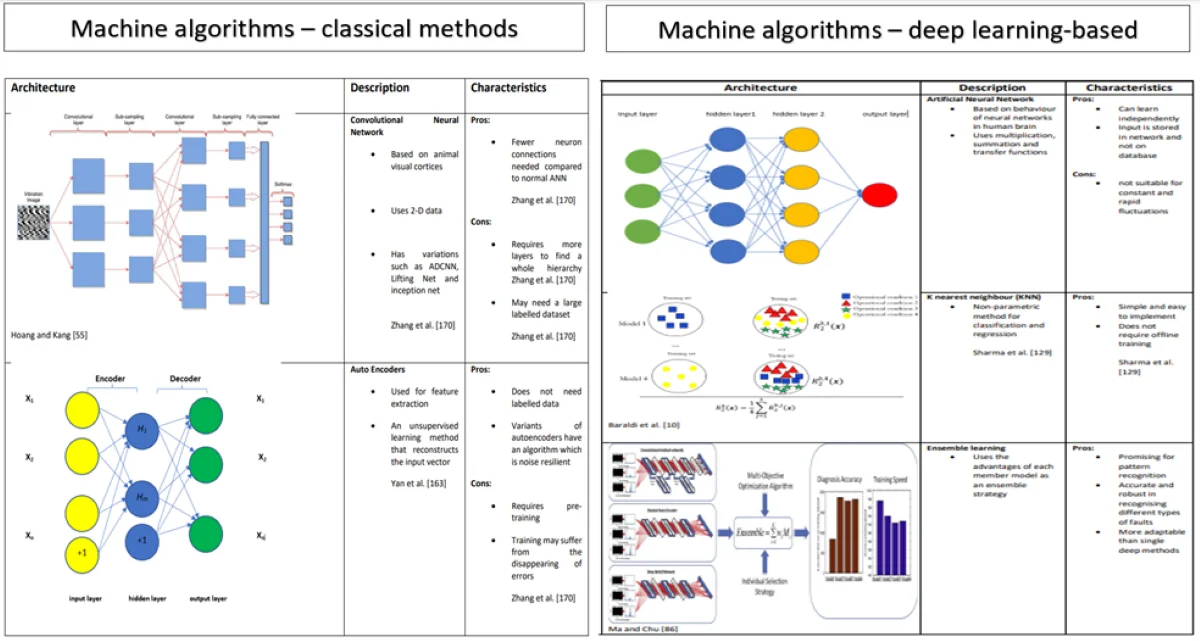
Table 1Summary of machine algorithms – classical methods – architecture, description and characteristics
Architecture | Description and characteristics |
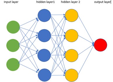 | Artificial Neural Network – Based on behaviour of neural networks in human brain – Uses multiplication, summation and transfer functions Pros: – Can learn independently – Input is stored in network and not on database Cons: – Not suitable for constant and rapid fluctuations |
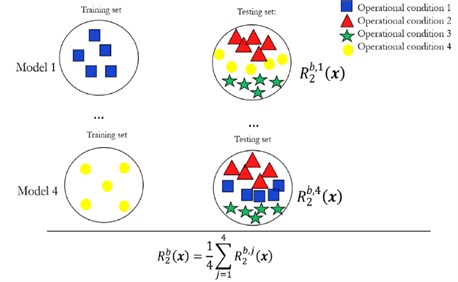 Baraldi et al. [51] | K Nearest Neighbour (KNN) – Non-parametric method for classification and regression Pros: – Simple and easy to implement – Does not require offline training Sharma et al. [53] |
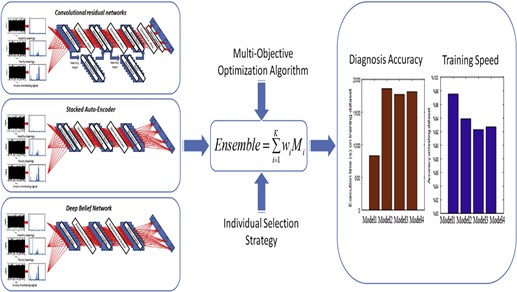 Ma and Chu [58] | Ensemble learning – Uses the advantages of each member model as an ensemble strategy Pros: – Promising for pattern recognition – Accurate and robust in recognising different types of faults – More adaptable than single deep methods |
 Abdi and Williams [2] | Principle Component Analysis (PCA) – Multivariate technique for analysing data tables – Describes intercorrelated quantitative dependent variables – Extracts important information from tables Pros: – Variance in the data is clear and explainable – Shows internal structure of data Abdi and Williams [2] |
In response to the issue of there being a broad application of technology for fault diagnosis and the associated limitation of the application of a single deep model, Ma and Chu [58] proposed an ensemble deep learning diagnosis method using multi-objective optimisation which was shown to be more adaptable in comparison to other ensemble and single deep methods. Furthermore, Xu et al. [59] recognised that most fault diagnosis methods find it difficult to learn representative features from raw data. In response to this issue, Xu et al. [59] proposed that deep learning with its ability to perform automatic feature extraction should be combined with ensemble learning, in this case, random forest (RF) ensemble learning, due to its ability to improve generalisation performance and accuracy of classifiers.
2.3.2. Deep learning-based approaches
Predicting remaining useful life (RUL) for rotating equipment is increasingly important for condition-based maintenance and it has been shown that deep learning prognosis methods are showing promise for bearings and gears. Deep belief networks and associated deep learning methods are a popular way for approaching the processing and analysis of big data and it has the ability to provide important features from the data that can be used for prediction of RUL [60]. Furthermore, due to the deep nature of these approaches, they can mine hidden information because of its multiple-layered structure [60].
Deep learning (DL) is an area within machine learning and is based on algorithms that are inspired by neural networks of the human brain. Deep learning is about improving the learning algorithm and making it easier to use [5]. A benefit of deep learning is that it can carry out automatic feature extraction from raw data through the ability of algorithms to learn representations using feature learning through exploiting the unknown structure of the input in order to reveal good representations [5]. It is important to note that DL approaches are essentially large neural networks that use large amounts of data and require large computers [5].
Furthermore, they are promising in the prediction of RUL for rotating equipment [61]. Concerning this, the deep learning approach proposed by Deutsch [61] was designed to overcome the limitations associated with signal processing and feature extraction requiring specific modelling and expertise. Specifically, their method which used vibration and acoustic emissions together with state transition modelling and a data-driven particle filter was validated using real bearing and gear run-to-failure test data [61].
It is important to make a distinction between the idea of deep learning and artificial network. The ‘deep’ refers to the idea that there many hidden layers in the network. The transition from the classic ‘shallow’ machine learning algorithms to deep learning is the result of many reasons. Firstly, data explosion, this is where there is an explosion in the amount of available data which means there has been a return of large-scale datasets in some domains. For the numerous applications which include diagnosing bearing faults these large data sets are not easily accessible, they are difficult to acquire which can also take some time.
With smaller datasets, classical machine learning algorithms can be equal in performance or even outperform DL networks. Where there is an increase in the data the deep learning can outperform classic machine learning algorithms. Secondly, there has been an evolution in algorithms as there has been an increase in techniques that have matured in control of the training process for deeper models for achieving greater speed and improved convergence as well as improvement in generalisation. Thirdly, there has been an evolution in hardware. To train deep networks extensive computation is required and performing this with the GPU accelerates the training process. GPU facilitates the parallel functioning of computational compatibility with computational capability together with deep neural networks, this makes GPU invaluable in training deep learning algorithms, furthermore, more powerful GPUs allow for quicker setup times.
These aforementioned factors allow the application of deep learning algorithms to a number of applications that are data related. There are a number of advantages associated with using deep learning algorithms and they include the following:
2.3.2.1. Convolutional neural network (CNN)
Convolutional neural networks are inspired by animal visual cortices and were first used for the detection of image patterns hierarchically including simple and complex features. The lower layers will have lower level features, and higher levels will detect features that are higher level, built on the lower level features.
About the architecture of CNN, the one-dimensional temporal raw data is taken from the accelerometers and are stacked in a two-dimensional vector-like image representation before a convolutional layer conducts feature extraction, thereafter, down sampling takes place in the pooling layer. This convolution and pooling combination are repeated numerous times to make the network deeper. The output from hidden layers is passed to connected layers and the output is then passed to a top classifier based on Sigmoid or Softmax for bearing fault detection.
Xu et al. [59] propose a fault diagnosis method based on CNN and random forest ensemble learning and achieved a high level of accuracy in bearing fault diagnosis and was an improvement on standard deep learning methods and traditional methods. CNN can learn features automatically from the inputted data and has the potential to overcome traditional methods [62].
Belmiloud et al. [5] use CNN as part of their method for determining RUL of rolling element bearings. Specifically, extracted features are fed into a deep CNN to construct a health indicator. Hoang and Kang [62] propose a method for bearing fault diagnosis using CNN where vibration signals are used directly as input and therefore, there is no need for feature extraction. Their method was found to be highly accurate even in noisy environments [62]. Specifically, the method transformed 1-D vibration signals into 2-D images taking advantage of CNN effectiveness in image classification [62]. The issue of noise was also addressed by Zhao et al. [39] who said that diagnosis is difficult for planetary gearboxes due to planetary noise. They propose a diagnosis method using synchrosqueezing transform (SST) and deep CNN together with envelope time-frequency representations, their method automatically recognised the planet bearing fault type and also removed interference from the time-frequency spectrum effectively avoiding misdiagnosis [39].
The problem of traditional time or frequency domain analysis, in that they cannot extract features effectively, has been addressed by Zhang et al. [63] who introduce an enhanced CNN method using short-time Fourier transform, scaled exponential linear unit and hierarchical regularisation, the results of their experimentation showed that the method had higher accuracy of fault diagnosis than other deep learning methods [63].
Liu et al. [64] solve the problem of information losses when using the fusion process through an ensemble CNN model for diagnosing bearing faults, specifically, the model used one multi-channel fusion convolutional neural network branch and two 1 dimensional CNN branches, the former extracts features from sensory data and the latter extracts from the inherent features which reduces the loss of information, overall the model was found to be more effective and robust than other models [ 64].
2.3.2.2. Auto-encoders
Autoencoders have their origins in pre-training methods used for artificial neural networks. After years of development this approach has become popular as a method of feature learning, furthermore, it has been described as being a greedy layer-wise method for pre-training.
An ANN is used to train the auto coder which is comprised of an encoder and a decoder whereby the encoder’s output is the input for the decoder. The mean square error between input and output as the loss function is taken by the ANN to generate the output through imitation of the output. Once the ANN has been trained the decoder is discarded and the encoder is retained. This means that the feature representation is the output of the encoder, and it is this that is used in the classifier in the next stage.
However, although autoencoders was an early approach, more modern and state-of-the-art approaches are more focussed on deep neural networks with many layers that employ a backpropagation algorithm [5]. Haidong et al. [65] presented a novel method for intelligent bearing fault diagnosis using ensemble learning which analyses experimental vibration signals together with a combination strategy to achieve an accurate diagnosis. The results showed the method removes the need to depend on manual feature extraction and overcomes limitations associated with deep learning models [65].
2.3.2.3. Deep belief network (DBN)
In deep learning, a deep belief network (DBN) is considered as a compilation of unsupervised networks, for example, restricted Boltzmann machines or auto-encoders, whereby the hidden layer of each sub-network acts as a visible layer which is used to train the DBN. Furthermore, for SAE the fused features are inputs into the DBN for the classification of faults.
Deutsch [61] validated deep learning prognosis methods using big data collected from bearing test rigs to determine bearing RUL predictions. One of the methods used by Deutsch [61] was the Deep Belief Network. Specifically, the DBN was trained using FFT features and upon completion of training a fine-tuning layer was added to the DBN, the results were promising as the approach added robustness to the architectures and reduced the probability of poor results [61].
Shao et al. [66] propose a novel continuous deep belief network optimised with the use of a genetic algorithm in order to adapt the characteristics of signals, the proposed method was tested using bearings and it was found to be superior in terms of accuracy and stability than traditional methods. Shen et al. [67] recognise the limitations of diagnosis mechanisms that use manual feature extraction, as a solution deep learning can learn representative features in the data without the need for much prior knowledge. Shen et al. [67] presented a new method for bearing fault analysis named hierarchical adaptive DBN optimised by using the Nesterov momentum, their model was validated using vibration signals from bearings and it was found that the method shows more satisfactory performance than conventional DBN and support vector machine [67].
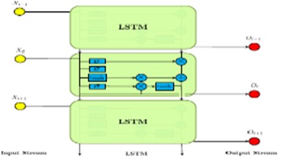
2.3.2.4. Recurrent neural network (RNN)
Data in the recurrent neural network method is processed in a recurrent behaviour as opposed to a feed-forward neural network. The flow path of this goes from the hidden layer back to the flow path when it is sequentially unrolled. Because it is a sequential model it can capture and model any sequential relationship that can be found in time series or sequential data [68].
A recent approach that used deep recurrent neural network (DRNN) was proposed by Jiang et al., [69] which used stack recurrent hidden layers as well as LSTM units, furthermore, an adaptive learning rate was also used to improve training performance. This approach returned high accuracy results of 94.75 % and 96.53 % [69]. Wu et al. [70] proposed a novel approach for fault prognosis using recurrent neural network, specifically, recurrent neural network was used with the degradation sequence of equipment, again with LSTM units, and showed significant performance in RUL prediction. Xie and Zhang [71] also recognised the beneficial potential of deep network neural algorithms, LSTM and recurrent neural network and proposed a novel approach for fault prognosis using LSTM based on the vibration signal of rotating equipment, the outcomes were successful in improving machine condition monitoring and health management.
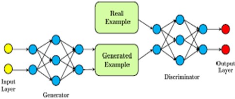
2.3.2.5. Generative adversarial network (GAN)
Goodfellow et al. [72] first proposed GAN in 2014 and is comprised of two parts which are the generator and the discriminator which compete with each other whereby tries to confuse while the latter tries to distinguish samples generated by the former. They are competing with each other to gain increased capability for imitating the original data samples and then to discriminate iteratively.
Table 2Summary of machine algorithms – deep learning-based approaches – architecture, description and characteristics
Architecture | Description and characteristics |
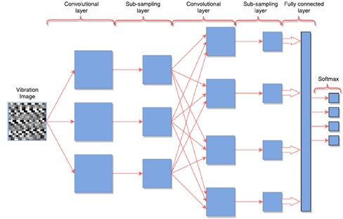 Hoang and Kang [62] | Convolutional Neural Network – Based on animal visual cortices – Uses 2-D data – Has variations such as ADCNN, Lifting Net and inception net Pros: – Fewer neuron connections needed compared to normal ANN Cons: – Requires more layers to find a whole hierarchy Zhang et al. [63] – May need a large labelled dataset Zhang et al. [63] |
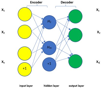 | Auto Encoders – Used for feature extraction – An unsupervised learning method that reconstructs the input vector Yan et al. [54] Pros: – Does not need labelled data – Variants of autoencoders have an algorithm which is noise resilient Cons: – Requires pre-training – Training may suffer from the disappearing of errors Zhang et al. [63] |
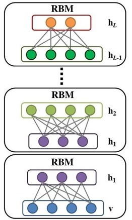 Lin et al. [73] | Deep Belief Network (DBN) – Built with RBMs – each hidden layer is the visible layer for the next – Undirected connection at the top two layers – Training is supervised or unsupervised Zhang et al. [63] Pros: – Can use layer by layer learning strategy to start the network – The likelihood is maximised through tractable inferences Zhang et al. [63] Cons: – Training can be computer-intensive and expensive due to initialisation and sampling |
 Zhang et al. [68] | Recurrent Neural Network – Analyses 1-D temporal or sequential data – Used for applications where output independent on previous computation Zhang et al. [63] Pros: – Can memorise sequential events – Can model time dependencies – Can receive inputs of variable lengths Zhang et al. [63] |
 Zhang et al. [68] | Generative Adversarial Network (GAN) – Uses a generator and a discriminator to generate images which imitate real photos – Augments data where labelled data is scarce Zhang et al. [63] Pros: – Does not need modification when moving to new applications – Does not have a deterministic bias Cons: – Training is unstable because requires finding Nash equilibrium – Difficult to learn how to create discrete data Zhang et al. [63] |
3. Prognosis
Achieving reliable and accurate prognosis is necessary for condition monitoring management, and is important for management of safety, scheduling and lowering costs [74]. Prognostics focuses on using automated methods for the detection, diagnosis, and analysis of system degradation and to estimate remaining useful life (RUL) within accepted operating parameters before failure occurs or performance degrades to intolerable levels. The success of a condition monitoring management strategy is dependent upon such automated procedures, which send out notices related to impending failure of equipment [75] to provide maintenance personnel with a lead time.
International Standard Organization (ISO) 13381-1 [76] defines prognostics as “the estimation of the Time to Failure (ETTF) and the risk of existence or later appearance of one or more failure modes”.
In the development of a prognostic method, the required outcome is the prediction of failure time [77, 78]. Predictions require that the system and associated condition processes are understood in addition to historic conditions that could affect the future behavior [79]. Because predictions are concerned with an event that is uncertain, approaches to prognostics consider basic assumptions about degradation characteristics, prognosis is based on the following four notions [80, 81]:
1) All systems degrade due to time and environmental factors.
2) Ageing and damage are monotonic processes that reveal themselves both physically and chemically.
3) Symptoms of ageing are detectable prior to failure
4) Symptoms of ageing can be correlated with a model of ageing and, therefore, the RUL of individual systems can be estimated.
At the initial stages of a system’s lifetime the components are working properly. Each operational function has a specific initial level of health, which is mostly stable at the early stages, which continues until an early incipient fault takes place. Over time as operation continues system failure becomes increasingly likely, which can lead to system damage and ultimately a catastrophic failure. It is important to note that system failure and catastrophic failure take place at different times. The early detection of such failures is critical in the estimation of the RUL. In order to detect fault characteristics it is necessary to have interactions between diagnostics and prognostics. The overall objective is to increase awareness of the state so that it takes place close to the point of the first incipient fault [82].
Degradation resulting from an initial system fault in a system continues to increase reaching a critical state that leads to system failure. The system begins with initial health and a variation that is acceptable and considered normal. The diagnostic representation here relates to the task of in-depth exploration of a failure that is a direct result of an initial leading symptom. Based on the location of this symptom, prognostics is about taking a multi-step approach before prediction [83].
Prognostic prediction is practiced between the initial failure detection and actual failure, where diagnostics are practiced [83]. Consequently, the goals of diagnostics and prognostics are somewhat different but carried out in the same field. Since both lifetime estimation methods are applied for condition monitoring, they both include stages for data acquisition and signal processing.
A variety of prognostic techniques with numerous tools and methods have been mentioned in the literature [84]. Current prognostic methods can be categorised into three general classes according to prediction and forecasting approaches: physics-based, data-based and hybrid approaches. Each approach has its particular disadvantages and advantages [85, 86].
3.1. Physics-based models
Physics-based models (PbM) describe the physics of the equipment and the failure mechanism [87]. In the physics-based approach the evolution of the degradation is defined and therefore, for this reason this approach is considered a degradation model [88]. Table 3 shows methods within the PbM prognostics approach. The mathematical models of degradation are usually used in applications that are associated with health levels. PbMs use a combination of formulas for fault growth together with knowledge related to the principles of damage mechanics. Using these models there is the assumption that where the mathematical model for component degradation is accurate then it can provide sufficient knowledge for prognostic outputs.
Table 3Physics based models
Approach | Description | Merits and limitations |
Paris and Erdogan Law [89] | Uses Paris’ Law [54] for crack growth modelling. Least-square scheme adapts model parameters to condition changes | It is assumed that defect area size is linearly correlated to vibration. In time series prediction, it is similar to single-step adaptation. The constants of materials are determined empirically |
Forman Law [90] | Crack growth is modelled by the Forman law of linear elastic fracture mechanics | It can relate monitoring data and crack growth. In order to examine the model, the assumption is required to be simplified. For complex condition, it is necessary to determine the model parameters. |
Paris law crack growth modeling with FEA [91, 92] | Finite Element Analysis with Paris & Erdogan Law for calculating stress and strain fields | Enables stress calculation. Performance accuracy is based on the crack size estimation of vibration data |
Contact Analysis [93] | Finite Element Analysis for calculating material stress field | It can determine the cycles to failure with damage mechanics principles. Different physics parameters are necessary to apply the model |
Fatigue spall initiation with Yu-Harris life equation [94] | Uses Yu-Harris bearing life equation for predicting spall initiation | Uses cumulative damage with consideration of operating conditions. Different physics parameters are necessary to apply the model |
A well know approach in PbM is Crack growth modelling. The Paris and Erdogan law [89] is employed in a number of applications to associate the stress intensity factor range with crack growth within the fatigue stress regime. The defect growth rate of rolling element bearings has been evaluated with a variation of Paris’ Law. This law states that defect growth is correlated with defect area. Predicted and actual defect sizes are compared followed by the application of a recursive least-square scheme to derive an adaptive prognostic model for defect growths [91, 92], however, a slight difference in a parameter may lead to a large prediction error. Li and Choi [91], and Li and Lee [92] presented a Paris’ law crack growth model using Finite Element Analysis (FEA), whereby estimation of stress is based on the size of the defect, bearing geometry, speed and load. The performance of this approach depends on crack size calculation accuracy using vibration data, and any calculations carried out are computationally-intensive so that the probability of an observation can be evaluated. Forman law of linear elastic fracture is another PbM model [90]. Oppenheimer and Loparo applied data from condition monitoring together with Forman law crack growth physics to life models. Because identification of the defect area size during operations is often instantaneous, this approach could be impractical for certain situations. Furthermore, assumptions may be oversimplified and there needs to be an examination of the model parameters before application [90].
Orsagh et al. presented a stochastic variation based on the Kotzalas-Harris model to for estimating failure progression and time-to-failure together with the Yu-Harris life equation for determining fatigue spall initiation. The current state of the bearing is estimated through calculating the time-to-spall initiation, followed by prediction of the future bearing health model [94, 95]. Marble and Morton [93] presented a PbM method for spall propagation using FEA to estimate spall size, material stress, rolling element speed and load. Their model can predict the number of cycles until failure with consideration of the principles of damage mechanics [93].
While there are numerous application domains and that there are differences between models, it is the case that the aforementioned models share common features making them appropriate for specific uses. Generally, PbM approaches are conventional and employ mathematical methods to understand failure modes [96]. In comparison to data-driven approaches PbM approaches are more accurate. However, PbM approaches may not be effective for estimating RUL in complex systems because it better for specific components rather than systems as a whole [86]. Furthermore, it is very difficult to describe the behavior of individual components within complex systems using unique mathematical equations. These approaches require a significant amount of experimentation [97], therefore, a specific PbM method for a specific system is not applicable to a different system.
3.2. Data-based model
In the data-based (DbP) approach monitoring data is processed in order to model prognostics instead of building mathematical models of system behaviours [98]. Data-based models involve precursors to failure and RUL by considering past data and estimating the output using monitoring data. One major advantage of data-based models is their simplicity in terms of calculation. These can be conducted using an algorithm to process past degradation patterns to estimate future degradation [78]. Although all data-based approaches are driven by data and - to some degree - use models they may be categorised as either model-based or data- driven [99].
In order to provide a RUL prediction, the prognostic model assumes that an accurate mathematical model for damage (or degradation) can use condition-monitoring data from the damage qualification step, which is initially progressed from system sensor measurements and the estimation algorithm. The model parameters for the remaining useful life prediction step are obtained from this designed combination model. The degradation model is expressed as a function of system data and model parameters. Damage classification and data are provided to the model while the damage model parameters of the estimation algorithm use these in order to describe the degradation behavior occurring in the system. Then, RUL is forecast based on the calculated model parameters [100].
Model-based prognostic methods include several techniques that employ dynamic models of the predicted process, such as Kalman and particle filtering method, autoregressive moving average (ARMA) techniques, and empirical methods [101]. Generally, these models are Bayesian-based, whereby the state of a process can be estimated using minimum prediction covariance derived from measurements. Kordestani et al. [102] proposed a method for fault prognosis based on neural networks and recursive Bayesian algorithm resulting in a high level of accuracy. They are capable of predicting current and future states of nonlinear systems and estimate the RUL based on deterioration trends before the asset arrives at the predefined threshold [100]. This reflects the fact that their involvement in the processes of RUL prediction is high. On the other hand, they do not directly learn from data, and they have shortcomings in terms of different operational trajectories.
Data-driven approaches for condition monitoring maintenance are calculated through analysing condition-monitoring data [74]. A prognostic approach is effective because its data discovery is simple and consistent in complex processes [86]. Data-driven models make it simple to integrate innovative approaches creating an inclusive prognostic approach [103]. A data driven approach to prognosis using a combination of principle component analysis with exponential degradation was proposed by Anis [104] using kurtosis and it was successful for prognostic of rotating shaft failure.
Common data-driven models in the prognostic field are explained in Table 4. These models provide prognostic applications with the ability to learn without being explicitly designed. Most of these approaches focus on the development of RUL prediction algorithms that can change when exposed to new but similar data. Conventional data-driven methods consist of simple forecast models including exponential smoothing, Gamma process [105, 106], and autoregressive models [107].
The main advantage of these techniques is that their implementation is simple, which can be carried out on a programmable estimator [117]. On the other hand, these basic projection techniques are based on the assumption that there is an underlying stability in the system being monitored, and they rely on historical performance to predict future degradation. This reliance is risky and can result in inaccurate forecasts when any trend changes or the data ends during a fluctuation. More complex systems such as Bayesian Networks [118, 120] and fuzzy logic systems [119, 120] have been developed for data-driven prognostic projections. These applications can extract useful knowledge from complex data in various forms but the prognostic accuracy in multi-step ahead predictions is limited in cases where long projections are expected but test trajectories are short.
Table 4Data driven prognostics
Approach | Description | Merits and limitations |
Artificial neural networks [108, 109] | Simulating biological neural network functions. They can learn the relationship between inputs and outputs | – Able to work on filtering, fitting, clustering, classification and prediction – No standard method |
Bayesian networks [110, 111] | A probabilistic graphical model that represents random variables and the structure of their conditional interdependency relations | – Less parameters required to calculate – Limited accuracy in complex systems |
Time series [112, 113] | Use ANNs to provide nonlinear projection | – Less parameters required to calculate – Limited accuracy in complex system |
Fuzzy logic [114] | Represent and process uncertainty to offer robust and noise tolerant models to make system complexity manageable | – Ability to deal with incomplete data and complexity. Compatible with human action – Not feasible to provide accurate RUL calculations |
Principal component analysis (PCA) [115, 50] | A dimensionality reduction model which transforms original features | – Reduces data sets to lower dimensions – Performance varies for different applications |
Similarity based prediction [10, 24, 116] | Uses pairwise distance evaluation for two degradation trajectories | – High level of prediction accuracy and reduction of prognostic risks – Requires large quantities of baseline trajectories |
Artificial Neural Networks (ANNs) are a widely used data-driven approach to prognostics [121, 52]. ANNs are computational algorithms that use data processing neurons to perform machine learning, this neural network is used as a connected computation of output values from the input data [122, 123]. ANNs are a key feature in establishing a set of interconnected relationships between inputs and desired outputs and they can be trained for performance [124].
Neural networks can effectively model systems comprising an extensive class of non-linear regression, non-linear dynamic systems, data reduction and discriminant models [125]. In certain applications such as to complex engineering systems, the measured data from the system may be imprecise, and the looked-for results may not be directly linked to the input data. In such cases, ANNs are suitable to model such systems where the precise relationship between input and output data is not known [126]. ANNs, therefore, are applicable to predictive algorithms for complicated systems and can be quicker and easier to use in comparison to other predictive methods. Thus, ANNs are a widely used data-driven prognostic method, and widely adopted across different disciplines.
Predictions using ANN can be difficult where there is insufficient knowledge about the degradation process [127, 128]. ANNs use actual sample points from the time series from the network modelling, specifically, the next value of the time series is predicted, without the need to feed back to input values [129, 130]. Where the prediction horizon is longer using multiple steps the ANN output should be fed back externally to the initial time series for a fixed number of steps; the regression components from these input series, previously formed from sample points from the initial time series, are gradually replaced by values that have already been predicted [128]. However, these replacements may lead to an imbalance in the predictions which may imitate training data [131]. However, ANNs provide sound computational mapping between raw data and outputs required in the network prediction [132].
3.3. Prognostics performance evaluation
Prognostic metrics could be seen as a standardised method of communication whereby users show their results and compare their findings [133]. Overtime due to numerous prognostic implementations in different disciplines, there have been metrics established for assessing forecasting performance including the work of Saxena, Leao, and Goebel [134, 135, 136]. These metrics sets validate prognostic application performance. Because they are concerned with applications with an availability of run-to-failure data and actual RUL is known, they are particularly useful for the model development stage whereby the metrics could be used for integration of prognostic procedures [133].
These metrics are defined mathematically and their relationship to prognostics design are presented in the equations that follow:
3.3.1. Error ()
Error is the deviation from a desired target [133]:
where is the estimated value (ETTF) and is the actual output value (ATTF). In this definition, the absolute error (AE) is the following:
3.3.2. Mean absolute error (MAE)
Where there is more than one instance, an average of the absolute error terms is calculated using the mean absolute error [137]. This measures the closeness of estimations to the actual outcomes:
3.3.3. Mean square error (MSE)
MSE is a risk function for calculating the average of the square values of the errors [137]. When the vector of these predictions is gained and the vectors of actual remaining useful life is available, the MSE can be calculated by:
3.4. Challenges of prognostics
Wang [117] said that successful prognostic applications are still difficult to find for complex engineering systems despite the fact there has been numerous algorithms proposed for calculating remaining useful life. There are numerous issues and misconceptions in the development of these algorithms which presents a challenge to prognostic applications used in complex systems. Furthermore, because data characteristics are complex, stochastic and exhibit nonlinear degradation patterns it is difficult to model systems accurately [138].
The challenges of prognostics and the associated requirements addressed in literature are provided here.
3.4.1. Lack of common data sources
Advanced prognostic techniques development is an active area of research, for a model to show promise there is need to collect data throughout the lifetime of a machine. As faults evolve further estimations by prognostic systems are required to detect these faults [139].
3.4.2. Uncertainty in predictions
There are a number of factors that influence system degradation and therefore, the associated noise, uncertainty and errors found in the data. Data-driven prognostics depend on the assumption that historical data can allow for a model for estimating remaining useful life, however, future operational conditions are unknown and require projection. However, it may not be possible to provide results when the length of the test data is short and there is a requirement for long term projections, in this case there may be a failure in prognostic accuracy.
3.4.3. Validation issues
Predicting remaining useful life is not the same as predicting future behaviour validated after a whole life cycle and reaching a real failure. If the dataset provides the actual time to failure the prediction can be validated using the metrics discussed in the above (2.10). Because metrics developed within forecasting are different from prognostic applications, they are a widely used method of validation and findings can be compared. Furthermore, metrics can be used to assess algorithmic performance in prognostic applications and are useful at the algorithm development stage whereby metric feedback is employed for fine tuning the prognostic algorithms [140]. However, where test data is short there is a higher risk of error, or if there are fluctuations resulting from operational conditions, the results can also be negatively affected.
4. Conclusions
In this paper, a comprehensive review of roller bearing diagnosis and prognosis has been reviewed. This review showed various techniques have been used in combination with vibration analysis for the diagnosis and prognosis of bearings element faults, however, most of these algorithms are valid for certain cases and cannot be generalised.
Although many researchers have addressed fault detection within roller element bearings there are many challenges facing fault detection. One of the most challenging scenarios is bearing fault detection where the vibration or acoustic signals are strongly masked by noise from more dominant components such as gears and shafts. An example of this scenario is the gearbox of a wind turbine, which presents difficulty for bearing fault detection. Therefore, this research aims to develop a diagnostic and prognostic tool to detect bearing faults and predict the remaining useful life under a strongly masked signal.
Although a large variety of prognostic models have been proposed and well reported in technical literature, an efficient prognostic methodology with accurate life prediction for real world application has yet to be developed. For accurate prognostics, it is essential to conduct prior analysis of the system’s degradation process, its failure patterns and to maintain a log of the history and condition of the machine throughout its life. Future research on the area of vibration analysis will address the gap related to prognosis capability through machine learning and propose a way to reduce dependency on training data to establish life prediction.
References
-
D. Abboud, M. Elbadaoui, W. A. Smith, and R. B. Randall, “Advanced bearing diagnostics: A comparative study of two powerful approaches,” Mechanical Systems and Signal Processing, Vol. 114, pp. 604–627, Jan. 2019, https://doi.org/10.1016/j.ymssp.2018.05.011
-
H. Abdi and L. J. Williams, “Principal component analysis,” Wiley Interdisciplinary Reviews: Computational Statistics, Vol. 2, No. 4, pp. 433–459, Jul. 2010, https://doi.org/10.1002/wics.101
-
“PeakVue Analysis for Antifriction Bearing Fault Detection,” White Paper Emerson, 2017.
-
O. Bektas, “An adaptive data filtering model for remaining useful life estimation,” Ph.D. Thesis, University of Warwick, 2018.
-
D. Belmiloud, T. Benkedjouh, M. Lachi, A. Laggoun, and J. P. Dron, “Deep convolutional neural networks for bearings failure prediction and temperature correlation,” Journal of Vibroengineering, Vol. 20, No. 8, pp. 2878–2891, Dec. 2018, https://doi.org/10.21595/jve.2018.19637
-
J. Ben Ali, B. Chebel-Morello, L. Saidi, S. Malinowski, and F. Fnaiech, “Accurate bearing remaining useful life prediction based on Weibull distribution and artificial neural network,” Mechanical Systems and Signal Processing, Vol. 56-57, pp. 150–172, May 2015, https://doi.org/10.1016/j.ymssp.2014.10.014
-
Y. Liao, P. Sun, B. Wang, and L. Qu, “Extraction of repetitive transients with frequency domain multipoint kurtosis for bearing fault diagnosis,” Measurement Science and Technology, Vol. 29, No. 5, p. 055012, May 2018, https://doi.org/10.1088/1361-6501/aaae99
-
M. Demetgul, K. Yildiz, S. Taskin, I. N. Tansel, and O. Yazicioglu, “Fault diagnosis on material handling system using feature selection and data mining techniques,” Measurement, Vol. 55, pp. 15–24, Sep. 2014, https://doi.org/10.1016/j.measurement.2014.04.037
-
Palmgren A., Ball and Roller Bearing Engineering. Philadelphia: S.H. Burbank and Co., 1947.
-
J. Qiu, B. B. Seth, S. Y. Liang, and C. Zhang, “damage mechanics approach for bearing lifetime prognostics,” Mechanical Systems and Signal Processing, Vol. 16, No. 5, pp. 817–829, Sep. 2002, https://doi.org/10.1006/mssp.2002.1483
-
P. Gupta and M. K. Pradhan, “Fault detection analysis in rolling element bearing: A review,” Materials Today: Proceedings, Vol. 4, No. 2, pp. 2085–2094, 2017, https://doi.org/10.1016/j.matpr.2017.02.054
-
I. Howard, “A Review of Rolling Element Bearing Vibration “Detection, Diagnosis and Prognosis”,” Department of Defence, Melbourne, 1994.
-
H. Saruhan, S. Sandemir, A. Çiçek, and I. Uygur, “Vibration analysis of rolling element bearings defects,” Journal of Applied Research and Technology, Vol. 12, No. 3, pp. 384–395, Jun. 2014, https://doi.org/10.1016/s1665-6423(14)71620-7
-
M. P. Norton and D. G. Karczub, Fundamentals of Noise and Vibration Analysis for Engineers. Cambridge University Press, 2003, https://doi.org/10.1017/cbo9781139163927
-
A. Rai and S. H. Upadhyay, “A review on signal processing techniques utilized in the fault diagnosis of rolling element bearings,” Tribology International, Vol. 96, pp. 289–306, Apr. 2016, https://doi.org/10.1016/j.triboint.2015.12.037
-
M. N. Jagdale and G. Diwakar, “A critical review of condition monitoring parameters for fault diagnosis of rolling element bearing,” in IOP Conference Series: Materials Science and Engineering, Vol. 455, p. 012090, Dec. 2018, https://doi.org/10.1088/1757-899x/455/1/012090
-
C. Scheffer and P. Girdha, Practical Machinery Vibration Analysis and Predictive Maintenance. Elsevier, 2004.
-
O. R. Seryasat, M. Aliyari Shoorehdeli, F. Honarvar, and A. Rahmani, “Multi-fault diagnosis of ball bearing using FFT, wavelet energy entropy mean and root mean square (RMS),” in 2010 IEEE International Conference on Systems, Man and Cybernetics – SMC, Oct. 2010, https://doi.org/10.1109/icsmc.2010.5642389
-
S. Mohanty, K. K. Gupta, and K. S. Raju, “Multi-channel vibro-acoustic fault analysis of ball bearing using wavelet based multi-scale principal component analysis,” in 2015 Twenty First National Conference on Communications (NCC), Feb. 2015, https://doi.org/10.1109/ncc.2015.7084916
-
J. Tian, C. Morillo, M. H. Azarian, and M. Pecht, “Motor bearing fault detection using spectral kurtosis-based feature extraction coupled with K-nearest neighbor distance analysis,” IEEE Transactions on Industrial Electronics, Vol. 63, No. 3, pp. 1793–1803, Mar. 2016, https://doi.org/10.1109/tie.2015.2509913
-
L. Saidi, J. Ben Ali, E. Bechhoefer, and M. Benbouzid, “Wind turbine high-speed shaft bearings health prognosis through a spectral Kurtosis-derived indices and SVR,” Applied Acoustics, Vol. 120, pp. 1–8, May 2017, https://doi.org/10.1016/j.apacoust.2017.01.005
-
Mitchell Lebold, Katherine Mcclintic, Robert Campbell, Carl Byington, and Kenneth Maynard, “Review of vibration analysis methods for gearbox diagnostics and prognostics,” in Proceedings of the 54th Meeting of the Society for Machinery Failure Prevention Technology, 2000.
-
R. B. W. Heng and M. J. M. Nor, “Statistical analysis of sound and vibration signals for monitoring rolling element bearing condition,” Applied Acoustics, Vol. 53, No. 1-3, pp. 211–226, Jan. 1998, https://doi.org/10.1016/s0003-682x(97)00018-2
-
H.-Q. Wang, W. Hou, G. Tang, H.-F. Yuan, Q.-L. Zhao, and X. Cao, “Fault detection enhancement in rolling element bearings via peak-based multiscale decomposition and envelope demodulation,” Mathematical Problems in Engineering, Vol. 2014, pp. 1–11, 2014, https://doi.org/10.1155/2014/329458
-
K. R. Al-Balushi, A. Addali, B. Charnley, and D. Mba, “Energy index technique for detection of Acoustic Emissions associated with incipient bearing failures,” Applied Acoustics, Vol. 71, No. 9, pp. 812–821, Sep. 2010, https://doi.org/10.1016/j.apacoust.2010.04.006
-
Q. Xu, S. Lu, W. Jia, and C. Jiang, “Imbalanced fault diagnosis of rotating machinery via multi-domain feature extraction and cost-sensitive learning,” Journal of Intelligent Manufacturing, Vol. 31, No. 6, pp. 1467–1481, Aug. 2020, https://doi.org/10.1007/s10845-019-01522-8
-
S. Yang. “Build up a Neural Network with Python.” Towardsdatascience.com. https://towardsdatascience.com/build-up-a-neural-network-with-python-7faea4561b31
-
J. R. Stack, T. G. Habetler, and R. G. Harley, “Fault classification and fault signature production for rolling element bearings in electric machines,” IEEE Transactions on Industry Applications, Vol. 40, No. 3, pp. 735–739, May 2004, https://doi.org/10.1109/tia.2004.827454
-
S. A. Abdusslam, “Detection and diagnosis of rolling element bearing faults using time encoded signal processing and recognition,” Ph.D. Thesis, University of Huddersfield, 2012.
-
R. R. Schoen and T. G. Habetler, “Effects of time-varying loads on rotor fault detection in induction machines,” IEEE Transactions on Industry Applications, Vol. 31, No. 4, pp. 900–906, 1995, https://doi.org/10.1109/28.395302
-
V. K. Rai and A. R. Mohanty, “Bearing fault diagnosis using FFT of intrinsic mode functions in Hilbert-Huang transform,” Mechanical Systems and Signal Processing, Vol. 21, No. 6, pp. 2607–2615, Aug. 2007, https://doi.org/10.1016/j.ymssp.2006.12.004
-
D. Gabor, “Theory of communication,” Journal of the Institution of Electrical Engineers – Part III: Radio and Communication Engineering, Vol. 93, No. 26, pp. 429–457, Nov. 1946.
-
M. Portnoff, “Time-frequency representation of digital signals and systems based on short-time Fourier analysis,” IEEE Transactions on Acoustics, Speech, and Signal Processing, Vol. 28, No. 1, pp. 55–69, Feb. 1980, https://doi.org/10.1109/tassp.1980.1163359
-
J.-H. Lee, J. Kim, and H.-J. Kim, “Development of enhanced Wigner-Ville distribution function,” Mechanical Systems and Signal Processing, Vol. 15, No. 2, pp. 367–398, Mar. 2001, https://doi.org/10.1006/mssp.2000.1365
-
C. Scheffer and P. Girdhar, Practical Machinery Vibration Analysis and Predictive Maintenance. Newnes, 2004.
-
G. Feng, H. Zhao, F. Gu, P. Needham, and A. D. Ball, “Efficient implementation of envelope analysis on resources limited wireless sensor nodes for accurate bearing fault diagnosis,” Measurement, Vol. 110, pp. 307–318, Nov. 2017, https://doi.org/10.1016/j.measurement.2017.07.009
-
R. B. Randall and J. Antoni, “Rolling element bearing diagnostics-A tutorial,” Mechanical Systems and Signal Processing, Vol. 25, No. 2, pp. 485–520, Feb. 2011, https://doi.org/10.1016/j.ymssp.2010.07.017
-
I. El-Thalji and E. Jantunen, “A summary of fault modelling and predictive health monitoring of rolling element bearings,” Mechanical Systems and Signal Processing, Vol. 60-61, pp. 252–272, Aug. 2015, https://doi.org/10.1016/j.ymssp.2015.02.008
-
D. Zhao, T. Wang, and F. Chu, “Deep convolutional neural network based planet bearing fault classification,” Computers in Industry, Vol. 107, pp. 59–66, May 2019, https://doi.org/10.1016/j.compind.2019.02.001
-
B. Li, M.-Y. Chow, Y. Tipsuwan, and J. C. Hung, “Neural-network-based motor rolling bearing fault diagnosis,” IEEE Transactions on Industrial Electronics, Vol. 47, No. 5, pp. 1060–1069, 2000, https://doi.org/10.1109/41.873214
-
T. Tung and B.-S. Yang, “Machine fault diagnosis and prognosis: the state of the art,” International Journal of Fluid Machinery and Systems, Vol. 2, No. 1, pp. 61–71, Mar. 2009, https://doi.org/10.5293/ijfms.2009.2.1.061
-
B. A. Paya, I. I. Esat, and M. N. M. Badi, “Artificial neural network based fault diagnostics of rotating machinery using wavelet transforms as a preprocessor,” Mechanical Systems and Signal Processing, Vol. 11, No. 5, pp. 751–765, Sep. 1997, https://doi.org/10.1006/mssp.1997.0090
-
J. P. Patel and S. H. Upadhyay, “Comparison between artificial neural network and support vector method for a fault diagnostics in rolling element bearings,” Procedia Engineering, Vol. 144, pp. 390–397, 2016, https://doi.org/10.1016/j.proeng.2016.05.148
-
Kai Goebel, Bhaskar Saha, and Abhinav Saxena, “A comparison of three data-driven techniques for prognostics,” in 62nd Meeting of the Society for Machinery Failure Prevention Technology (MFPT), pp. 119–131, Jan. 2008.
-
N. A. Aditiya, Z. Darojah, D. R. Sanggar, and M. R. Dharmawan, “Fault diagnosis system of rotating machines using continuous wavelet transform and artificial neural network,” in 2017 International Electronics Symposium on Knowledge Creation and Intelligent Computing (IES-KCIC), Sep. 2017, https://doi.org/10.1109/kcic.2017.8228582
-
M. J. Gómez, C. Castejón, and J. C. García-Prada, “Automatic condition monitoring system for crack detection in rotating machinery,” Reliability Engineering and System Safety, Vol. 152, pp. 239–247, Aug. 2016, https://doi.org/10.1016/j.ress.2016.03.013
-
M. Beretta, Y. Vidal, J. Sepulveda, O. Porro, and J. Cusidó, “Improved ensemble learning for wind turbine main bearing fault diagnosis,” Applied Sciences, Vol. 11, No. 16, p. 7523, Aug. 2021, https://doi.org/10.3390/app11167523
-
E. P. de Moura, C. R. Souto, A. A. Silva, and M. A. S. Irmão, “Evaluation of principal component analysis and neural network performance for bearing fault diagnosis from vibration signal processed by RS and DF analyses,” Mechanical Systems and Signal Processing, Vol. 25, No. 5, pp. 1765–1772, Jul. 2011, https://doi.org/10.1016/j.ymssp.2010.11.021
-
Y.-J. Park, S.-K. S. Fan, and C.-Y. Hsu, “A review on fault detection and process diagnostics in industrial processes,” Processes, Vol. 8, No. 9, p. 1123, Sep. 2020, https://doi.org/10.3390/pr8091123
-
F. Wang, X. Chen, B. Dun, B. Wang, D. Yan, and H. Zhu, “Rolling bearing reliability assessment via kernel principal component analysis and Weibull proportional Hazard model,” Shock and Vibration, Vol. 2017, pp. 1–11, 2017, https://doi.org/10.1155/2017/6184190
-
P. Baraldi, F. Cannarile, F. Di Maio, and E. Zio, “Hierarchical k-nearest neighbours classification and binary differential evolution for fault diagnostics of automotive bearings operating under variable conditions,” Engineering Applications of Artificial Intelligence, Vol. 56, pp. 1–13, Nov. 2016, https://doi.org/10.1016/j.engappai.2016.08.011
-
H. Wang, Z. Yu, and L. Guo, “Real-time online fault diagnosis of rolling bearings based on KNN algorithm,” in Journal of Physics: Conference Series, Vol. 1486, p. 032019, Apr. 2020, https://doi.org/10.1088/1742-6596/1486/3/032019
-
A. Sharma, R. Jigyasu, L. Mathew, and S. Chatterji, “Bearing fault diagnosis using weighted K-nearest neighbor,” in 2018 2nd International Conference on Trends in Electronics and Informatics (ICOEI), pp. 1132–1137, May 2018, https://doi.org/10.1109/icoei.2018.8553800
-
Z. Yan, X. Yuan, F. Zhou, Y. Song, Q. Xu, and Y. Shao, “Fault diagnosis based on a stacked sparse auto-encoder network and KNN classifier,” in 2019 Chinese Automation Congress (CAC), Nov. 2019, https://doi.org/10.1109/cac48633.2019.8996595
-
B. Zhang, L. Zhang, and J. Xu, “Remaining useful life prediction for rolling element bearing based on ensemble learning,” Chemical Engineering Transactions, Vol. 33, pp. 157–162, Jul. 2013, https://doi.org/10.3303/cet1333027
-
T. Liang, S. Wu, W. Duan, and R. Zhang, “Bearing fault diagnosis based on improved ensemble learning and deep belief network,” in Journal of Physics: Conference Series, Vol. 1074, p. 012154, Sep. 2018, https://doi.org/10.1088/1742-6596/1074/1/012154
-
X. Li, H. Jiang, M. Niu, and R. Wang, “An enhanced selective ensemble deep learning method for rolling bearing fault diagnosis with beetle antennae search algorithm,” Mechanical Systems and Signal Processing, Vol. 142, p. 106752, Aug. 2020, https://doi.org/10.1016/j.ymssp.2020.106752
-
S. Ma and F. Chu, “Ensemble deep learning-based fault diagnosis of rotor bearing systems,” Computers in Industry, Vol. 105, pp. 143–152, Feb. 2019, https://doi.org/10.1016/j.compind.2018.12.012
-
G. Xu, M. Liu, Z. Jiang, D. Söffker, and W. Shen, “Bearing fault diagnosis method based on deep convolutional neural network and random forest ensemble learning,” Sensors, Vol. 19, No. 5, p. 1088, Mar. 2019, https://doi.org/10.3390/s19051088
-
G. Box, G. Reinsel, and G. Jenkins, Time Series Analysis, 4th ed. Wiley, 2008.
-
J. Deutsch, “Development of deep learning based prognostics for rotating component,” in Annual Doctoral Symposium, 2017.
-
D.-T. Hoang and H.-J. Kang, “Rolling element bearing fault diagnosis using convolutional neural network and vibration image,” Cognitive Systems Research, Vol. 53, pp. 42–50, Jan. 2019, https://doi.org/10.1016/j.cogsys.2018.03.002
-
Y. Zhang, K. Xing, R. Bai, D. Sun, and Z. Meng, “An enhanced convolutional neural network for bearing fault diagnosis based on time-frequency image,” Measurement, Vol. 157, p. 107667, Jun. 2020, https://doi.org/10.1016/j.measurement.2020.107667
-
Y. Liu, X. Yan, C.-A. Zhang, and W. Liu, “An ensemble convolutional neural networks for bearing fault diagnosis using multi-sensor data,” Sensors, Vol. 19, No. 23, p. 5300, Dec. 2019, https://doi.org/10.3390/s19235300
-
S. Haidong, J. Hongkai, Z. Ke, W. Dongdong, and L. Xingqiu, “A novel tracking deep wavelet auto-encoder method for intelligent fault diagnosis of electric locomotive bearings,” Mechanical Systems and Signal Processing, Vol. 110, pp. 193–209, Sep. 2018, https://doi.org/10.1016/j.ymssp.2018.03.011
-
H. Shao, H. Jiang, X. Li, and T. Liang, “Rolling bearing fault detection using continuous deep belief network with locally linear embedding,” Computers in Industry, Vol. 96, pp. 27–39, Apr. 2018, https://doi.org/10.1016/j.compind.2018.01.005
-
C. Shen, J. Xie, D. Wang, X. Jiang, J. Shi, and Z. Zhu, “Improved hierarchical adaptive deep belief network for bearing fault diagnosis,” Applied Sciences, Vol. 9, No. 16, p. 3374, Aug. 2019, https://doi.org/10.3390/app9163374
-
S. Zhang, S. Zhang, B. Wang, and T. G. Habetler, “Deep learning algorithms for bearing fault diagnostics-a comprehensive review,” IEEE Access, Vol. 8, pp. 29857–29881, 2020, https://doi.org/10.1109/access.2020.2972859
-
H. Jiang, X. Li, H. Shao, and K. Zhao, “Intelligent fault diagnosis of rolling bearings using an improved deep recurrent neural network,” Measurement Science and Technology, Vol. 29, No. 6, p. 065107, Jun. 2018, https://doi.org/10.1088/1361-6501/aab945
-
Q. Wu, K. Ding, and B. Huang, “Approach for fault prognosis using recurrent neural network,” Journal of Intelligent Manufacturing, Vol. 31, No. 7, pp. 1621–1633, Oct. 2020, https://doi.org/10.1007/s10845-018-1428-5
-
Y. Xie and T. Zhang, “A long short term memory recurrent neural network approach for rotating machinery fault prognosis,” in 2018 IEEE CSAA Guidance, Navigation and Control Conference (GNCC), pp. 1–6, Aug. 2018, https://doi.org/10.1109/gncc42960.2018.9018860
-
I. Goodfellow et al., “Generative adversarial nets,” Advances in Neural Information Processing Systems, Vol. 27, 2014.
-
P. Lin, S.-W. Fu, S.-S. Wang, Y.-H. Lai, and Y. Tsao, “Maximum entropy learning with deep belief networks,” Entropy, Vol. 18, No. 7, p. 251, Jul. 2016, https://doi.org/10.3390/e18070251
-
Y. Peng, M. Dong, and M. J. Zuo, “Current status of machine prognostics in condition-based maintenance: a review,” The International Journal of Advanced Manufacturing Technology, Vol. 50, No. 1-4, pp. 297–313, Sep. 2010, https://doi.org/10.1007/s00170-009-2482-0
-
S. Butler, “Prognostic algorithms for condition monitoring and remaining useful life estimation,” Ph.D. Thesis, National University of Ireland, 2012.
-
D. A. Tobon-Mejia, K. Medjaher, and N. Zerhouni, “The ISO 13381-1 Standard’s failure prognostics process through an example,” in 2010 Prognostics and System Health Management Conference (PHM), pp. 1–12, Jan. 2010, https://doi.org/10.1109/phm.2010.5413482
-
C. T. Leonard and M. G. Pecht, “Improved techniques for cost effective electronics,” in Annual Reliability and Maintainability Symposium. 1991, pp. 174–182, 1991, https://doi.org/10.1109/arms.1991.154432
-
M. G. Pecht, “Prognostics and health management of electronics,” in Encyclopedia of Structural Health Monitoring, Chichester, UK: John Wiley & Sons, Ltd, 2008, https://doi.org/10.1002/9780470061626.shm118
-
S. Sankararaman and K. Goebel, “Remaining useful life estimation in prognosis: An uncertainty propagation problem,” in AIAA Infotech Conference 2013, Aug. 2014.
-
S. Uckun, K. Goebel, and P. J. F. Lucas, “Standardizing research methods for prognostics,” in 2008 International Conference on Prognostics and Health Management (PHM), Oct. 2008, https://doi.org/10.1109/phm.2008.4711437
-
M. Baptista, S. Sankararaman, I. P. de Medeiros, C. Nascimento, H. Prendinger, and E. M. P. Henriques, “Forecasting fault events for predictive maintenance using data-driven techniques and ARMA modeling,” Computers and Industrial Engineering, Vol. 115, pp. 41–53, Jan. 2018, https://doi.org/10.1016/j.cie.2017.10.033
-
A. Hess, G. Calvello, P. Frith, S. J. Engel, and D. Hoitsma, “Challenges, issues, and lessons learned chasing the “Big P”: real predictive prognostics part 2,” 2006 IEEE Aerospace Conference, 2006, https://doi.org/10.1109/aero.2006.1656124
-
J. Lee, F. Wu, W. Zhao, M. Ghaffari, L. Liao, and D. Siegel, “Prognostics and health management design for rotary machinery systems-Reviews, methodology and applications,” Mechanical Systems and Signal Processing, Vol. 42, No. 1-2, pp. 314–334, Jan. 2014, https://doi.org/10.1016/j.ymssp.2013.06.004
-
S. T. Kandukuri, A. Klausen, H. R. Karimi, and K. G. Robbersmyr, “A review of diagnostics and prognostics of low-speed machinery towards wind turbine farm-level health management,” Renewable and Sustainable Energy Reviews, Vol. 53, pp. 697–708, Jan. 2016, https://doi.org/10.1016/j.rser.2015.08.061
-
J. Z. Sikorska, M. Hodkiewicz, and L. Ma, “Prognostic modelling options for remaining useful life estimation by industry,” Mechanical Systems and Signal Processing, Vol. 25, No. 5, pp. 1803–1836, Jul. 2011, https://doi.org/10.1016/j.ymssp.2010.11.018
-
A. Heng, S. Zhang, A. C. C. Tan, and J. Mathew, “Rotating machinery prognostics: State of the art, challenges and opportunities,” Mechanical Systems and Signal Processing, Vol. 23, No. 3, pp. 724–739, Apr. 2009, https://doi.org/10.1016/j.ymssp.2008.06.009
-
O. F. Eker, F. Camci, and I. K. Jennions, “A Similarity-based prognostics approach for remaining useful life prediction,” PHM Society European Conference, Vol. 2, No. 1, 2014, https://doi.org/10.36001/phme.2014.v2i1.1479
-
T. Johns, N. C. Street, J. W. Sheppard, M. A. Kaufman, and T. J. Wilmering, “IEEE standards for prognostics and health management,” in IEEE Autotestcon 2008, Vol. 24, No. 9, pp. 97–103, Sep. 2008, https://doi.org/10.1109/autest.2008.4662592
-
Y. Li, T. R. Kurfess, and S. Y. Liang, “Stochastic prognostics for rolling element bearings,” Mechanical Systems and Signal Processing, Vol. 14, No. 5, pp. 747–762, Sep. 2000, https://doi.org/10.1006/mssp.2000.1301
-
C. H. Oppenheimer and K. A. Loparo, “Physically based diagnosis and prognosis of cracked rotor shafts,” AeroSense 2002, Vol. 4733, pp. 122–132, Jul. 2002, https://doi.org/10.1117/12.475502
-
C. J. Li and S. Choi, “Spur gear root fatigue crack prognosis via crack diagnosis and fracture mechanics,” in Proceedings of the 56th Meeting of the Society of Mechanical Failures Prevention Technology, pp. 311–320, 2002.
-
C. J. Li and H. Lee, “Gear fatigue crack prognosis using embedded model, gear dynamic model and fracture mechanics,” Mechanical Systems and Signal Processing, Vol. 19, No. 4, pp. 836–846, Jul. 2005, https://doi.org/10.1016/j.ymssp.2004.06.007
-
S. Marble and B. P. Morton, “Predicting the remaining life of propulsion system bearings,” in 2006 IEEE Aerospace Conference, 2006, https://doi.org/10.1109/aero.2006.1656121
-
R. F. Orsagh, J. Sheldon, and C. J. Klenke, “Prognostics/diagnostics for gas turbine engine bearings,” in 2003 IEEE Aerospace (Cat. No.03TH8652), pp. 159–167, 2003, https://doi.org/10.1109/aero.2003.1234152
-
R. Orsagh, M. Roemer, J. Sheldon, and C. J. Klenke, “A comprehensive prognostics approach for predicting gas turbine engine bearing life,” in ASME Turbo Expo 2004: Power for Land, Sea, and Air, pp. 777–785, Jan. 2004, https://doi.org/10.1115/gt2004-53965
-
G. Vachtsevanos, F. Lewis, M. Roemer, A. Hess, and B. Wu, Intelligent Fault Diagnosis and Prognosis for Engineering Systems. Hoboken: Wiley, 2006.
-
L. Liao and F. Kottig, “Review of hybrid prognostics approaches for remaining useful life prediction of engineered systems, and an application to battery life prediction,” IEEE Transactions on Reliability, Vol. 63, No. 1, pp. 191–207, Mar. 2014, https://doi.org/10.1109/tr.2014.2299152
-
M. S. Kan, A. C. C. Tan, and J. Mathew, “A review on prognostic techniques for non-stationary and non-linear rotating systems,” Mechanical Systems and Signal Processing, Vol. 62-63, pp. 1–20, Oct. 2015, https://doi.org/10.1016/j.ymssp.2015.02.016
-
M. J. Daigle and K. Goebel, “Model-based prognostics with concurrent damage progression processes,” IEEE Transactions on Systems, Man, and Cybernetics: Systems, Vol. 43, No. 3, pp. 535–546, May 2013, https://doi.org/10.1109/tsmca.2012.2207109
-
D. An, J.-H. Choi, and N. H. Kim, “Prognostics 101: A tutorial for particle filter-based prognostics algorithm using Matlab,” Reliability Engineering and System Safety, Vol. 115, pp. 161–169, Jul. 2013, https://doi.org/10.1016/j.ress.2013.02.019
-
D. C. Swanson, “A general prognostic tracking algorithm for predictive maintenance,” in 2001 IEEE Aerospace Conference Proceedings, 2000, https://doi.org/10.1109/aero.2001.931317
-
M. Kordestani, M. F. Samadi, and M. Saif, “A new hybrid fault prognosis method for MFS systems based on distributed neural networks and recursive Bayesian algorithm,” IEEE Systems Journal, Vol. 14, No. 4, pp. 5407–5416, Dec. 2020, https://doi.org/10.1109/jsyst.2020.2986162
-
C. S. Byington, M. Watson, and D. Edwards, “Data-driven neural network methodology to remaining life predictions for aircraft actuator components,” in 2004 IEEE Aerospace Conference Proceedings (IEEE Cat. No.04TH8720), 2004, https://doi.org/10.1109/aero.2004.1368175
-
M. D. Anis, “Towards remaining useful life prediction in rotating machine fault prognosis: an exponential degradation model,” in 2018 Condition Monitoring and Diagnosis (CMD), Sep. 2018, https://doi.org/10.1109/cmd.2018.8535765
-
X.-S. Si, W. Wang, C.-H. Hu, and D.-H. Zhou, “Remaining useful life estimation – A review on the statistical data driven approaches,” European Journal of Operational Research, Vol. 213, No. 1, pp. 1–14, Aug. 2011, https://doi.org/10.1016/j.ejor.2010.11.018
-
J. Lawless and M. Crowder, “Covariates and random effects in a gamma process model with application to degradation and failure,” Lifetime Data Analysis, Vol. 10, No. 3, pp. 213–227, Sep. 2004, https://doi.org/10.1023/b:lida.0000036389.14073.dd
-
K. Kazmierczak, “Application of autoregressive prognostic techniques in diagnostics,” in Proceedings of the Vehicle Diagnostics Conference, Mar. 1983.
-
K. Rostek, Morytko, and A. Jankowska, “Early detection and prediction of leaks in fluidized-bed boilers using artificial neural networks,” Energy, Vol. 89, pp. 914–923, Sep. 2015, https://doi.org/10.1016/j.energy.2015.06.042
-
S. Schrader, M.-O. Gewaltig, U. Körner, and E. Körner, “Cortext: A columnar model of bottom-up and top-down processing in the neocortex,” Neural Networks, Vol. 22, No. 8, pp. 1055–1070, Oct. 2009, https://doi.org/10.1016/j.neunet.2009.07.021
-
Todd Andrew Stephenson, “An introduction to Bayesian network theory and usage,” IDIAP, Technical Reports, Jan. 2000.
-
D. Heckerman, “Bayesian networks for data mining,” Data Mining and Knowledge Discovery, Vol. 1, No. 1, pp. 79–119, 1997, https://doi.org/10.1023/a:1009730122752
-
Z. Tian, L. Wong, and N. Safaei, “A neural network approach for remaining useful life prediction utilizing both failure and suspension histories,” Mechanical Systems and Signal Processing, Vol. 24, No. 5, pp. 1542–1555, Jul. 2010, https://doi.org/10.1016/j.ymssp.2009.11.005
-
William W. S. Wei, The Oxford Handbook of Quantitative Methods in Psychology: Vol. 2: Statistical Analysis. Oxford University Press, 2013, https://doi.org/10.1093/oxfordhb/9780199934898.013.0022
-
S. Mofizul Islam, T. Wu, and G. Ledwich, “A novel fuzzy logic approach to transformer fault diagnosis,” IEEE Transactions on Dielectrics and Electrical Insulation, Vol. 7, No. 2, pp. 177–186, Apr. 2000, https://doi.org/10.1109/94.841806
-
P.-J. Vlok, M. Wnek, and M. Zygmunt, “Utilising statistical residual life estimates of bearings to quantify the influence of preventive maintenance actions,” Mechanical Systems and Signal Processing, Vol. 18, No. 4, pp. 833–847, Jul. 2004, https://doi.org/10.1016/j.ymssp.2003.09.003
-
P. Wang and G. Vachtsevanos, “Fault prognostics using dynamic wavelet neural networks,” Artificial Intelligence for Engineering Design, Analysis and Manufacturing, Vol. 15, No. 4, pp. 349–365, Sep. 2001, https://doi.org/10.1017/s0890060401154089
-
Tianyi Wang, “Trajectory similarity based prediction for remaining useful life estimation,” Ph.D. Thesis, University of Cincinnati, 2010.
-
W. Teng, C. Han, Y. Hu, X. Cheng, L. Song, and Y. Liu, “A robust model-based approach for bearing remaining useful life prognosis in wind turbines,” IEEE Access, Vol. 8, pp. 47133–47143, 2020, https://doi.org/10.1109/access.2020.2978301
-
I. Y. Tumer and E. M. Huff, “Analysis of triaxial vibration data for health monitoring of helicopter gearboxes,” Journal of Vibration and Acoustics, Vol. 125, No. 1, pp. 120–128, Jan. 2003, https://doi.org/10.1115/1.1526130
-
Fagang Zhao, Jin Chen, Lei Guo, and Xinglin Li, “Neuro-fuzzy based condition prediction of bearing health,” Journal of Vibration and Control, Vol. 15, No. 7, pp. 1079–1091, Jul. 2009, https://doi.org/10.1177/1077546309102665
-
W. Q. Wang, M. F. Golnaraghi, and F. Ismail, “Prognosis of machine health condition using neuro-fuzzy systems,” Mechanical Systems and Signal Processing, Vol. 18, No. 4, pp. 813–831, Jul. 2004, https://doi.org/10.1016/s0888-3270(03)00079-7
-
C. M. Bishop, Neural Networks for Pattern Recognition. Oxford University Press, 1995.
-
C. Byington et al., “IECEC2001-ET-08 electrochemical cell diagnostics using online impedance measurement, state estimation and data fusion techniques,” in Proceedings of the Intersociety Energy Conversion Engineering Conference, 2001.
-
Z. Tian, “An artificial neural network method for remaining useful life prediction of equipment subject to condition monitoring,” Journal of Intelligent Manufacturing, Vol. 23, No. 2, pp. 227–237, Apr. 2012, https://doi.org/10.1007/s10845-009-0356-9
-
W. Sarle, “Neural networks and statistical models,” in Proceedings of the Nineteenth Annual SAS Users Group International Conference, 1994.
-
N. Murata, S. Yoshizawa, and S. Amari, “Network information criterion-determining the number of hidden units for an artificial neural network model,” IEEE Transactions on Neural Networks, Vol. 5, No. 6, pp. 865–872, 1994, https://doi.org/10.1109/72.329683
-
J. M. P. Menezes and G. A. Barreto, “Long-term time series prediction with the NARX network: An empirical evaluation,” Neurocomputing, Vol. 71, No. 16-18, pp. 3335–3343, Oct. 2008, https://doi.org/10.1016/j.neucom.2008.01.030
-
A. Sorjamaa, J. Hao, N. Reyhani, Y. Ji, and A. Lendasse, “Methodology for long-term prediction of time series,” Neurocomputing, Vol. 70, No. 16-18, pp. 2861–2869, Oct. 2007, https://doi.org/10.1016/j.neucom.2006.06.015
-
R. Zemouri, R. Gouriveau, and N. Zerhouni, “Defining and applying prediction performance metrics on a recurrent NARX time series model,” Neurocomputing, Vol. 73, No. 13-15, pp. 2506–2521, Aug. 2010, https://doi.org/10.1016/j.neucom.2010.06.005
-
A. Grigorievskiy, Y. Miche, A.-M. Ventelä, E. Séverin, and A. Lendasse, “Long-term time series prediction using OP-ELM,” Neural Networks, Vol. 51, pp. 50–56, Mar. 2014, https://doi.org/10.1016/j.neunet.2013.12.002
-
E. Sutrisno, H. Oh, A. S. S. Vasan, and M. Pecht, “Estimation of remaining useful life of ball bearings using data driven methodologies,” in 2012 IEEE Conference on Prognostics and Health Management (PHM), Jun. 2012, https://doi.org/10.1109/icphm.2012.6299548
-
H. Demuth, Neural Network Toolbox. The MathWorks, Inc, 2002.
-
A. Saxena, J. Celaya, B. Saha, S. Saha, and K. Goebel, “Metrics for offline evaluation of prognostic performance,” International Journal of Prognostics and Health Management, Vol. 1, No. 1, Mar. 2021, https://doi.org/10.36001/ijphm.2010.v1i1.1336
-
A. Saxena et al., “Metrics for evaluating performance of prognostic techniques,” in 2008 International Conference on Prognostics and Health Management (PHM), Oct. 2008, https://doi.org/10.1109/phm.2008.4711436
-
B. P. Leao, T. Yoneyama, G. C. Rocha, and K. T. Fitzgibbon, “Prognostics performance metrics and their relation to requirements, design, verification and cost-benefit,” in 2008 International Conference on Prognostics and Health Management (PHM), Oct. 2008, https://doi.org/10.1109/phm.2008.4711429
-
Abhinav Saxena, Jose Celaya, Bhaskar Saha, Sankalita Saha, and Kai Goebel, “On applying the prognostic performance metrics,” Annual Conference of the PHM Society, Vol. 1, No. 1, 2009.
-
R. J. Hyndman and A. B. Koehler, “Another look at measures of forecast accuracy,” International Journal of Forecasting, Vol. 22, No. 4, pp. 679–688, Oct. 2006, https://doi.org/10.1016/j.ijforecast.2006.03.001
-
F. Eker, “A hybrid prognostic methodology and its application to well-controlled engineering systems,” Ph.D. Thesis, Cranfield University, 2013.
-
T. Brotherton, P. Grabill, D. Wroblewski, R. Friend, B. Sotomayer, and J. Berry, “A testbed for data fusion for engine diagnostics and prognostics,” in 2002 IEEE Aerospace Conference, 2002, https://doi.org/10.1109/aero.2002.1036145
-
A. N. Srivastava and J. Han, Machine Learning and Knowledge Discovery for Engineering Systems Health Management. CRC Press, 2011.
About this article

