Abstract
Aiming at the problem of endpoint effect in empirical mode decomposition (EMD), the application method of support vector regression machine (SVRM) in EMD extension data prediction is studied. Firstly, the basic principle, data extension method and parameter setting of SVRM are introduced. Secondly, several application methods of SVRM in EMD extension are studied to analyze and verify the operational efficiency and decomposition accuracy characteristics of each method respectively. Finally, the proposed extension method based on SVRM extreme value point prediction can greatly improve the operation efficiency of SVRM long time extension. The simulation signal analysis shows that the SVRM extreme point prediction extension method not only improves the accuracy and reliability of EMD decomposition, but also effectively inhibits the end-point effect phenomenon, significantly reduces the SVRM extension time, and improves the practicability of EMD method.
1. Introduction
Empirical mode decomposition (EMD) in the processing of nonlinear, non-stationary signals has unique adaptability, so that it has been in-depth research and application, but the endpoint effect has been restricting the spread of EMD application in seismic signals, structural analysis and mechanical fault diagnosis field, but the endpoint effect has been restricting the spread of EMD application [1].
The extension method based on the original data is based on the data itself, which is fast and suitable for long time extension. Huang et al. found the problem of endpoint effect when the EMD method was proposed, proposed the characteristic wave method and applied for a patent [2]. Mirror closed extension method is simple in operation and efficient in the extension of long data. However, the truncated signal at the extreme value will cause partial information loss, so it is not suitable for the processing of short data, and it is not effective when the signal symmetry is poor [3]. The sinusoidal matching method alleviates the problem of end-point effect to a certain extent, but in practical application, the constructed waveform is difficult to reflect the change trend of the signal, and its practicability is poor [4]. The waveform matching method maintains the change trend of the original signal well, and has a good effect on the signal with regular waveform and strong periodicity [5]. However, for the signal with bad periodicity, it may be difficult to find the wavelet with high matching degree. The algorithm based on data prediction has high general accuracy and good extension smoothness, but the application range of EMD is affected due to the large amount of computation [6]. The prediction algorithm based on neural network has a high accuracy, but it requires a lot of training samples and takes too long learning time to carry out real-time online processing [7]. The adaptive autoregressive model processing method has high operational efficiency, but the autoregressive model itself belongs to linear operation, and its application effect to non-stationary signals is poor [8]. On the basis of summarizing the principle of endpoint effect in EMD decomposition, this paper studies the application of Support vector machine regression (SVRM) in EMD extension data prediction based on the problem of endpoint effect in empirical mode decomposition (EMD).
2. Overview of SVRM theory
2.1. Data series extension method of SVRM
After constructing the regression training model of SVRM, the data points can be extended forward and backward by using it. The following is an example to introduce the extension method and steps of SVRM:
(a) Construct the training set according to the existing data sequence.
For a given data sequence , ,…, , where is the number of sampling points in the data column. Firstly, the number of training samples is determined, and a training set , where , , .
(b) Construct regression model.
The regression model is constructed according to the above method.
(c) Predict the first sequence value.
The first predicted value outside the boundary can be obtained:
(d) Step by step iteration to obtain predictive sequence values.
Then let as the new boundary point of the original data, the extension value of the second data sequence can be obtained, and so on. According to the required extension length , the whole extension sequence can be obtained , ,…, , the value of any extension is:
where, the value of any extension is .
2.2. Setting of extension parameters
The extension precision of SVRM increases with the increase of the number of samples, while the operation efficiency decreases with the increase of the number of samples. Therefore, in order to ensure the extension accuracy, the number of samples must be increased or decreased with the extension length . Set . In general, short time extension requires a higher extension accuracy, and is set as a smaller value. In the case of long time extension, the extension accuracy requirements can be appropriately reduced, and a larger can be selected to improve the operational efficiency. Specifically, the length between the signal extreme points is taken as the reference, so that:
where, is the distance between extremum points; and are respectively the moment of the th minimum and maximum value of the signal, is the sample length coefficient, 0.
3. EMD extension algorithm based on SVRM
In order to prevent the endpoint effect of EMD from spreading into the signal as the decomposition progresses, we always hope to obtain the data extension of sufficient length accurately in a relatively short time. In order to ensure the prediction accuracy of data, sufficient sample quantity is required, while a long extension requires a large sample quantity, which will result in low computational efficiency. Therefore, improving the efficiency of SVRM extension in EMD application has become an urgent problem to be solved.
3.1. EMD primary extension algorithm based on SVRM
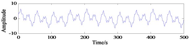
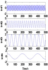
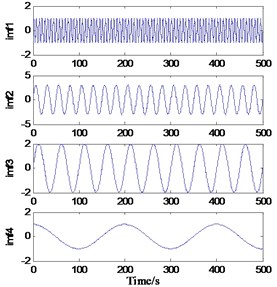
The primary extension method refers to the IMF which only conducts primary extension of data before EMD decomposition and then truncates the extension part of the obtained decomposition results to obtain the original data. The characteristic of this method is that the whole decomposition process only needs primary extension, the algorithm is simple to implement, and there is no accumulation of error caused by repeated extension. The simulation signal is taken as an example, and the waveform is shown in Fig. 1. The SVRM method is adopted to carry out a long extension, and then EMD decomposition. Sample length and extension length were controlled by adjusting the values of and . The decomposition of can is shown in Fig. 2:
Fig. 1Waveform of simulated signal y2t
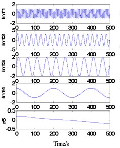
As shown in Fig. 2(a), when 1 and 5, the sample length 16 and the extension length 90, the decomposition results show large deformation at both ends, and the endpoint effect is not effectively contained. When 5 and 5, the sample length increases to 90. At this time, the decomposition results also show a large deformation at both ends, that is, the endpoint effect is effectively contained without the increase of the sample length. It can be inferred that when 5, the extension length is too short, so the endpoint effect is not effectively contained outside the real signal. When 1 and 20, the extension length increases to 320 points, and the decomposition results are greatly improved. There is no obvious distortion at the end points, but residual term is generated. It can be inferred that when 1, the regression model cannot accurately predict the signal trend due to the small sample data. When 5 and 20, the sample length increased to 80 points. At this time, a more accurate decomposition result was obtained, but the running time of the program increased to 71.8776 s.
3.2. EMD decomposition and extension simultaneously based on SVRM
In order to avoid the problem of operation efficiency caused by SVRM long time extension, an effective method is to make full use of the accuracy of SVRM short time extension, and adopt appropriate algorithm to avoid long time extension. The effective method is to decompose while extension. The idea is to conduct a short time extension with a length of more than two extreme points before each screening of EMD, and then cut off the extension part after generating the envelope. Since the algorithm needs to be extended before each screening, it only needs to extend a pair (a maximum value and a minimum value) above the extreme point at both ends of the signal each time. Repeated simulation experiments verify that, under the same conditions, when the two ends extend more than four extreme points respectively, the decomposition results will no longer change significantly. In order to ensure the decomposition accuracy, the method of extending four extreme points at both ends is adopted in this paper. Set 4, then the EMD processing results of are shown in Fig. 3.
Fig. 2Decomposition of simulated signal after one extension
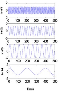
a)1, 5, 0.7648 s
b)5, 5, 22.2817 s
c)1, 20, 2.4462 s
d)5, 20, 71.8776 s

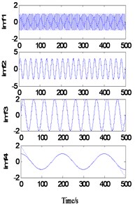
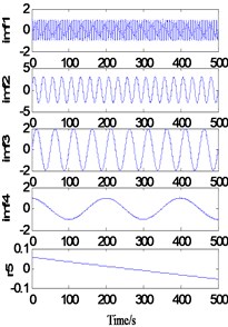
In the Fig. 3, when the sample is 10, residual terms are generated in the decomposition result; when the sample is increased to 20, the decomposition result reaches a very high precision, and at this time, the whole decomposition process takes only 0.9045 s.
It can be seen from Fig. 3 that when 1, due to the small sample number and poor extension accuracy, the endpoint effect is restrained to some extent, but residual terms appear. When 2, a relatively accurate decomposition result was obtained, and the operation time reached 388.2863 s.
Fig. 3Decomposition of simulated signal after decomposition and extension simultaneously
a)1, 4, 139.4893 s
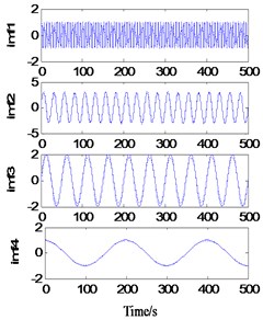
b)2, 4, 388.2863 s

3.3. EMD continuation based on SVRM extremum prediction
The extremum forecast and continuation process, SVRM extremum predict continuation of sample sequence is extremum sequence of original signal, so the methods require original signal have enough number of extreme value (experiments show general may not be less than 6), when the signal extremum number is small, SVRM based on hard less extreme value point accurately predict epitaxial signal extremum position and value. It should be noted that, with the progress of EMD decomposition, the frequency components of the obtained components gradually decrease. If this method is used for side decomposition and side continuation, the phenomenon of inaccurate continuation may occur in the low-frequency stage due to the small number of extreme points. Therefore, this method is more suitable for the previous continuation of decomposition. The decomposition results are shown in Fig. 4.
Fig. 4EMD results of continuation prediction based on SVRM extreme value
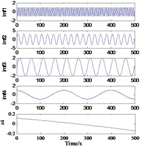
a)10, 30, 0.7239 s
b)20, 30, 0.9045 s

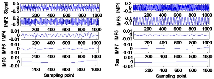
In order to verify the validity of the effect of the endpoint effect and the practical practicability of the actual hydraulic system, the sampling frequency of the measured hydraulic system is analyzed, and the sampling frequency is 5 kHz, and the sampling point is 2048. The results of EMD continuation based on SVRM extremum prediction results are as shown in the Fig. 5. The weak at both ends, and the similar components of the frequency are not visible in the endpoints, and the model of the IMF component is obviously suppressed.
Fig. 5EMD results of hydraulic fault signal
4. Conclusions
Based on the application of SVRM in EMD continuation, this paper introduces the prediction principle of SVRM, and proposes a method to set the extension length and sample number with the signal extremum scale. The advantages and disadvantages of various SVRM application methods in EMD continuation are analyzed from the Angle of decomposition accuracy and efficiency.
References
-
Huang N. E., Shen Zheng, Long S. R., et al. The empirical mode decomposition and the Hilbert spectrum for nonlinear and nonstationary time series analysis. Proceedings of the Royal Society of London. Series A, Mathematical and Physical Sciences, Vol. 454, Issue 1971, 1998, p. 903-995.
-
Huang N. E., Wu M. L., Qu W. D. Applications of Hilbert-Huang transform to non-stationary financial time series analysis. Applied Stochastic Models in Business and industry, Vol. 19, Issue 3, 2003, p. 245-268.
-
Zhao Jinping Improvement of the mirror extending in empirical mode decomposition method and the technology for eliminating frequency mixing. High Technology Letters, Vol. 8, Issue 3, 2002, p. 40-47.
-
Lin D. C., Guo Z. L., An F. P., et al. Elimination of end effects in empirical mode decomposition by mirror image coupled with sup ort vector regression. Mechanical Systems and Signal Processing, Vol. 31, 2012, p. 13-28.
-
Tang B. P., Dong S. J., Song T. Method for eliminating mode mixing of empirical mode decomposition based on the revised blind source separation. Signal Processing, Vol. 92, Issue 1, 2012, p. 248-258.
-
Guhathakurta K., Mukherjee I., Chowdhury A. R. Empirical mode decomposition analysis of two different financial time series and their comparison. Chaos, Solitons and Fractals, Vol. 37, 2008, p. 1214-1227.
-
Yu L., Wang S., Lai K. K. Forecasting crude oil price with an EMD-based neural network ensemble learning paradigm. Energy Economics, Vol. 30, 2008, p. 2623-2635.
-
Wu F. J., Qu L. S. An improved method for restraining the end effect in empirical mode decomposition and its applications to the fault diagnosis of large rotating machinery. Journal of Sound and Vibration, Vol. 314, 2008, p. 586-602.
About this article

