Abstract
The algorithm for solving the Riemann problem is considered in detail in the article. The statement of the Riemann problem is presented. The limitations of the algorithm described above and possible ways to overcome them are revealed. An improvement in the solution of the Riemann problem algorithm is presented.
1. Introduction
The use of front tracking methods for the modeling of a three-phase flow in a porous medium was initially difficult due to the fact that there are no analytical solutions to the corresponding Riemann problem, a particular case of the Cauchy problem, when the initial condition is two constants separated by a single break [1]. Most of the pre-existing solutions of the Riemann problem with respect to three-phase filtration were limited to the consideration of simplified functions of relative permeability, in which the relative permeability for each phase depends only on the saturation of this phase. But even when this restriction was weakened, and the relative permeabilities could be functions of all saturation, in published works on this topic, there were only general guidelines for constructing the solution (see, for example, [2]). Only relatively recently in [3-5] a complete set of solutions of such a problem was presented under the condition that certain limitations are imposed on the function of relative permeability. Moreover, the paper proposed effective algorithms for finding solutions. They were based on a correction-correction strategy in conjunction with the iterative Newton-Raphson procedure, which provided quadratic convergence. Since the solution of the Cauchy problem usually requires the solution of a large number of Riemann problems, the presence of a general and highly efficient solver of Riemann is topical. An example of such a solver is described in [1], which is also based on the use of the predictor-corrector strategy, the algorithm of which is as follows:
1. Set the left and right states: and .
2. Set the initial approximation and the trial solution: , , .
3. Find the solution for a given configuration and update the wave structure: .
4. Verify the admissibility (monotonic increase in wave velocities): if , then set a new initial approximation and designate the solution as incorrect 0.
5. Check the convergence of the algorithm: if , then stop, otherwise assign and . Go to step 3.
Given the left and right states and , accordingly, the algorithm solves the Riemann problem by determining the intermediate state and the types of waves , connecting the three constants. The algorithm begins by setting the initial approximation of the intermediate state and assuming that the trial solution is, i.e. consists of two rarefaction waves. This choice ensures that the expected intermediate state will be inside the triangle of saturation [1]. The core of the algorithm is Section 3, in which the following two actions are performed:
1. An intermediate state is determined for a given trial wave structure and initial approximation .
2. It is found out which structure of the solution waves could be for the newly calculated intermediate state. The wave type is displayed separately for each of the families ( 1,2). Although in order to obtain a reliable implementation, this step must be developed with caution, the idea is quite simple: the admissible discontinuity of the family must satisfy the Lax entropy condition; if the discontinuity is not permissible, and the constant states connected with the help of the wave of the family are located on one side relatively , then we have a rarefaction wave of the family, otherwise a mixed wave.
Due to the fact that for some saturation states the solution must include detached branches of the phase Hugoniot set, it is not sufficient to verify the admissibility of only individual waves. If there are gaps in the solution, then you need to make sure that they form an increasing sequence of wave velocities, i.e. that [1]. The algorithm finishes work if the trial wave structure is admissible . Otherwise, the values of the intermediate state and wave structure are updated to the calculated values. It is believed that the rarefaction and discontinuity curves in the phase space are usually located close enough to each other, so the position of the intermediate state is not very sensitive to the type of solution, and the procedure converges, as a rule, in one iteration [1].
2. Modeling results of the algorithm improvement for Riemann problem solving
Developed in [1, 3], the algorithms for solving the Riemann problem with respect to one-dimensional three-phase filtering in most cases yield fairly fast convergent results with a given accuracy. However, when testing the proposed approaches by setting randomly inside the triple diagram of left and right states, some limitations of the algorithm described above and possible ways of overcoming them were revealed.
We consider the case and for which in Fig. 1 shows the basic sets and curves that form the solution.
Fig. 1Integral curves and Hugoniot sets for Sl=0,40,6T and Sr=0,050,9T
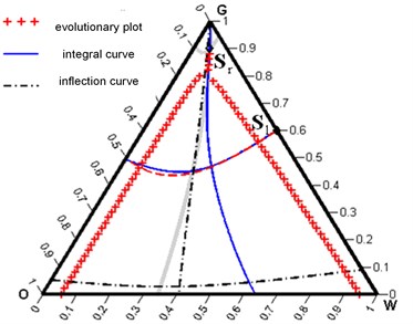
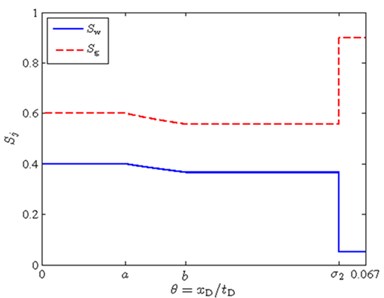
It can be seen that the Hugoniot phase set for a state includes a detached branch, and the integral curve and the local Hugoniot curve of the second family below the same state differ significantly from each other and actually are on opposite sides relative to . The above algorithm will determine the intermediate state and the appropriate solution structure for . In other words, the intersection of integral curves gives an unsuccessful initial approximation for finding the correct . As a result, the algorithm leads to an inadmissible solution, shown in Fig. 2.
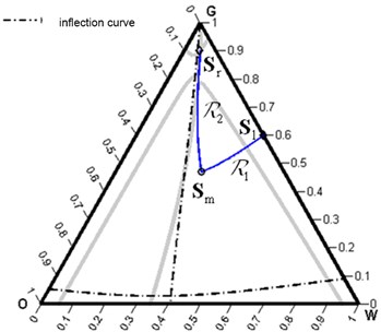
Fig. 2Inadmissible solution in the form of a R1R2 wave
a)
b)
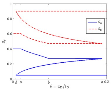
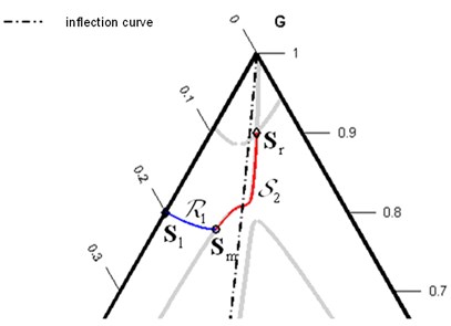
Fig. 3A feasible solution in the form R1S2 wave
a)
b)
The problem lies in point 4 of the algorithm, which assumes that possible solutions that are unsuccessful from the point of view of monotonous increase in the wave velocities of the structure of the solution given by the function will arise only if there is an obligatory presence of discontinuities in the solution. The example in Fig. 1 shows that this is not so. Verify the feasibility of the solution for all possible wave configurations in the solution. In this case, a really physically correct solution, shown in Fig. 3.
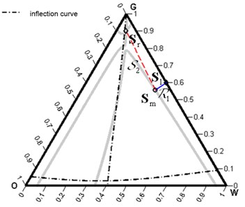
Another case where the initial trial solution is an unsuccessful choice is shown in Fig. 4, where an enlarged fragment of the triangular diagram is shown for the same right-hand state as in Fig. 1, but with the left state . The algorithm will find a solution for , namely , and will establish that with such an intermediate state the probable structure of the solution . Indeed, this is possible because and are on opposite sides relatively .
However, in the construction of the first wave , and then finding the intersection of the curves and in accordance with the procedures described in [3], a situation arises where the refined intermediate state at the next step of the iteration will be on the same side relative to the left state. It is clear that in this case there is no sense in continuing to build a wave, since the following condition must necessarily be satisfied: the left and right states must lie on opposite sides of the inflection curve .
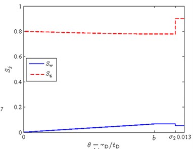
In fact, it is quite easy to resolve this situation. It is necessary to designate the proposed structure of the solution as incorrect and to refine it in accordance with a new approximation . So, for the example given in Fig. 4, after the construction of the -wave was not possible, after the refinement, the following structure of the solution was chosen: which turned out to be suitable, which is confirmed by Fig. 5.
Fig. 4Integral curves and Hugoniot sets for Sl=0,40,6T and Sr=0,050,9T
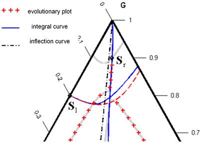
Fig. 5A feasible solution in the form R1S2 wave
a)
b)
3. Conclusions
The solution of the Riemann problem on an infinite domain and piecewise constant initial conditions with a single discontinuity is extremely important for practical application. A lot of laboratory experiments actually reproduce the conditions of the Riemann problem: initially the medium has homogeneous saturations, and the proportion of injected fluids remains constant during the experiment. The solution of the Riemann problem also gives information on the structure of the system of equations and can be used as a building block for obtaining solutions to problems with more complicated initial and boundary conditions. An improved algorithm for solving the Riemann problem is presented.
References
-
Lie K. A., Juanes R. A front-tracking method for the simulation of three-phase flow in porous media. Computational Geosciences, Vol. 9, Issue 1, 2005, p. 29-59.
-
Aziz H., Settari E. Mathematical Modeling of Reservoir Systems. Institute of Computer Research, Мoskow, Izhevsk, 2004, p. 416.
-
Juanes R. Displacement Theory and Multiscale Numerical Modeling of Three-Phase Flow in Porous Media. Ph.D. Thesis, University of California, Berkeley, California, 2003.
-
Hemming R. V. Numerical Methods for Scientists and Engineers. Nauka, Moskow, 1972, p. 400.
-
Anraku T., Horne R. N. Discrimination between reservoir models in well test analysis. SPE Formation Evaluation, Vol. 10, Issue 2, 1995, p. 114-121.
About this article

