Inference of the optimal probability distribution model for geotechnical parameters by using Weibull and NID distributions

1. Introduction

Due to the natural attributes of rock materials, the complexity of the geological environment and the randomness of external loading (such as impact loads, seismic response, vibratory action, etc.), uncertainty is inevitable in geotechnical engineering [1-3]. To quantitatively evaluate the influence of this uncertainty, reliability analysis has been widely used in many fields of geotechnical engineering [4, 5], such as slope reliability [6-12], tunnel and underground cavity reliability [13, 14], etc. In the reliability analysis of geotechnical engineering under quasi-static loads or vibrations loads, the inference of optimal probability density function (PDF) or cumulative distribution function (CDF) of a geotechnical parameter is one of the most essential tasks; this is the first step in a reliability analysis and plays a central role in ensuring the precision and accuracy of the geotechnical reliability analysis [15, 16]. Through the comparison and selection of the classical distributions (normal distribution, log-normal distribution, Weibull distribution, gamma distribution, etc.), some previous studies have shown that many geotechnical parameters will accept a Weibull distribution as the optimal PDFs [17-20]. However, there are some unsolved issues in the application process of the Weibull distribution. The specific PDF forms of the Weibull distribution are not uniform (including the two-parameter, three-parameter and mixed Weibull distributions), and the parameters of the Weibull distribution, such as the shape parameter $m$, the scale parameter $\sigma$ or the position parameter $\mu$, are sometimes difficult to estimate. In addition, the total cumulative probability value of the Weibull distribution is generally less than 1.0000 because its defined interval does not match the actual finite interval of geotechnical parameters. It is necessary to study the inference method, which more accurately represents the actual distribution.

In recent years, the normal information diffusion (NID) theory has been the focus of the attention of many scholars and has been further developed by C. F. Huang et al. [21, 22]. NID theory provides a new way to study function approximation based on the information assignment method of a fuzzy set. In NID theory, the original information is directly transferred to the fuzzy relation in a way that avoids calculation of the membership function and preserves the original information contained in the original data as much as possible. Due to the advantages of the information diffusion principle, NID theory has been successfully applied to some fields of study, especially to natural disaster and risk assessment [23-25].

In this paper, NID theory was introduced to fit the optimal PDFs or CDFs of geotechnical parameters. Two geotechnical parameters, the strength of a rock mass affected by acid [26] and the average wind speed [27], were used as examples to investigate the goodness of fit in a comparative analysis of the NID distribution and Weibull distribution. In addition, the effect of the sample size on the fitting accuracy of these two distributions was also illustrated with MC simulation samples. The results show that NID distribution can make full use of the sample information to deduce the PDFs of the geotechnical parameters and that its fit is more accurate than that of the Weibull distribution.

2. Weibull distribution

In mathematical statistics, the Weibull distribution has a range of function forms, including the two-parameter, three-parameter and mixed Weibull distributions, which are widely used in various fields of research. The specific Weibull distribution function is determined by the shape parameter $m$, the scale parameter $\sigma$ and the position parameter $\mu$. Among these parameters, the most important parameter is the shape parameter, which determines the basic shape of the PDF curve. In addition, the scale parameter effects the scaling of the PDF curve. In the geotechnical engineering reliability, the two-parameter Weibull distribution is one of the most commonly used models [18, 19]. The PDF of the two-parameter Weibull distribution can be written as Eq. (1):

where $F(\cdot )$ denotes the cumulative distribution function. $m$ and $\sigma$ is the shape parameter and the scale parameter, respectively.

3. NID distribution

The basic principle of the NID distribution was developed by C. F. Huang [21], and a brief introduction is as follows.

Suppose that the PDF of a random variable $x$ is $f\left(x\right)$; then, $\mu \left(x\right)$ is defined as a Borel measurable function in $(-\mathrm{\infty },+\mathrm{\infty })$. The diffusion estimation of $f\left(x\right)$ can be expressed as Eq. (2):

where ${\mathrm{\Delta }}_n>$ 0 is defined as the window width and $\mu \left(x\right)$ is defined as a diffusion function $f\left(x\right)$. According to the information diffusion process, $\mu \left(x\right)$ can be written as Eq. (3):

Substituting Eq. (3) into Eq. (2), the normal information diffusion function can be written as follows Eq. (4):

where $h$ denotes the window width of the standard normal diffusion function $\mu \left(x\right)$, $n$ denotes the sample size of a random variable, $x_i$ ($i=$ 1, 2, 3, …) is the observed values of the random variable, and $x_{max}$ and $x_{min}$ are the maximum value and minimum value of $x_i$, respectively. According to the principle of choosing the nearest normal information diffusion, $h=\gamma \left(x_{max}-x_{min}\right)/(n-1)$, in which $\gamma$ is related to the sample size (Table 4). When the sample size is greater than or equal to 17, $\gamma$ is always equal to 1.420693101. The details of the information diffusion process are discussed in Huang’s study [22].

4. Fitting comparison of the NID distribution and Weibull distribution

4.3. Distribution parameters of the actual samples

The parameters of the NID distribution and Weibull distribution are given in Tables 4 and 5. The window width $hs$ of the NID distribution for the samples 1# and 2# are 5.9196 and 0.2743, respectively. The distribution parameters of sample 1# are obtained from [26] and 1# belongs to the two-parameter Weibull distribution because its position parameter $\mu$ is equal to zero. For determining the distribution parameters of sample 2#, compared with the fitting goodness of the three-parameter Weibull distribution obtained from [27] and two-parameter Weibull distribution obtained from the maximum likelihood estimation (MLE) method, as shown in Fig. 1(b), it was found that the two-parameter Weibull distribution can be accepted as the probability distribution more accurately than the three-parameter Weibull distribution.

Table 3The interval values of the actual samples

Sample	Size	Mean	Standard deviation	Skewness	Truncated interval
					Left	Right
1#	19	131.8947	18.9616	–0.1464	72.2338	188.7797
2#	30	7.1467	1.5684	0.3385	2.4415	12.3827

Table 4The parameters of the NID distributions

Sample	$n$	$x_{max}$	$x_{min}$	$\gamma$	$h$
1#	19	167	92	1.420693101	5.9196
2#	30	10.2	4.6	1.420693101	0.2743

Table 5The results of the K-S test values and CDF values

Sample	distribution parameters			Comparison of the K-S test results			CDF values
	$m$	$\sigma$	$\mu$	Weibull	NID	$D_{n,0.05}$	Weibull	NID
1#	7.2500	140.3000	0.0000	0.0969	0.0683	0.3100	0.9917	1.0000
2# (2P)	5.0339	7.7777	0.0000	0.1495	0.0576	0.2420	0.9966	1.0000
2# (3P)	2.1754	3.4344	3.4395	0.2141	0.0576	0.2420	0.9996	1.0000
Note: 2P and 3P denote the two-parameter and three-parameter Weibull distributions, respectively

Fig. 1Comparative K-S test results of the actual sample data

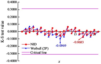
a) Sample 1#

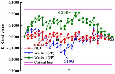
b) Sample 2#

4.5. Comparison of the fitting probability distribution curves

The empirical cumulative frequency curves and theoretical CDF curves for the two actual sample datasets are given Fig. 2. Within the truncated interval, the goodness of fit of the NID distribution is much more accurate than that of the Weibull distribution.

Fig. 2Comparative CDF curves of the actual sample datasets

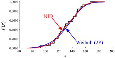
a) Sample 1#

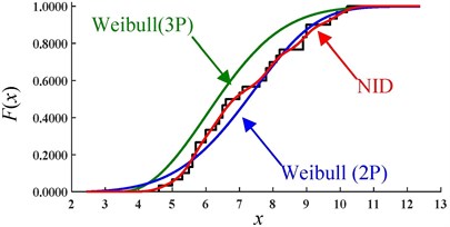
b) Sample 2#

Fig. 3Comparative PDF curves of the actual sample datasets

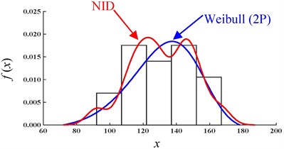
a) Sample 1#

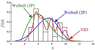
b) Sample 2#

The PDF curves and histograms for the two actual samples are also given in Fig. 3. Due to the uncertainty in and complexity of the geotechnical parameters, the distributions of the actual samples often present a certain fluctuation. As one of the single-peak distributions, the Weibull distribution cannot be used to describe the characteristics of the fluctuation in the actual distribution. However, the NID distribution is very flexible and can be used to describe this fluctuation (Fig. 3).

To summarize, whether for CDF curves or PDF curves, the NID distribution will approximate the actual distribution more accurately than the Weibull distribution will. The superiority of the NID distribution can be further confirmed by describing the actual distributions of the geotechnical parameters.

5. Effect of sample size on fitting accuracy

Considering that the sample sizes obtained in actual geotechnical engineering are generally small, to study the effect of the sample size on the fitting accuracy with the NID distribution and Weibull distribution, eight simulated samples of different sizes were produced by using the MC method in this paper. Two known Weibull distributions estimated by samples 1# and 2#, WBL1# (7.2500, 140.3000) and WBL2# (5.0339, 7.7777), were used as the generating functions in the MC method, and the simulated sample sizes are 15, 20, 30, 50, 100, 200, 500, and 1000 (partial sample datasets are shown in Table 6).

The K-S test was first used to test the validity of the NID distribution and Weibull distribution. The K-S test results and critical values under different sizes are given in Table 7 and Table 8. The effect of the sample size on the K-S test results is shown in Fig. 4. With an increase in the sample size, the K-S test results of the two fitting methods gradually decrease and tend to converge to the horizontal axis. However, compared with the K-S test results of the Weibull distribution, those of the NID distribution are much lower. The convergence speed and stability and the K-S test results of the NID distribution are all superior to those of the Weibull distribution.

In addition, the chi-square test was used to investigate the fitting ability for all the samples with a sample size larger than 50. The chi-square test results for a 95 % confidence level are shown in Table 9.

Fig. 4K-S test results of the simulated data with the sample size

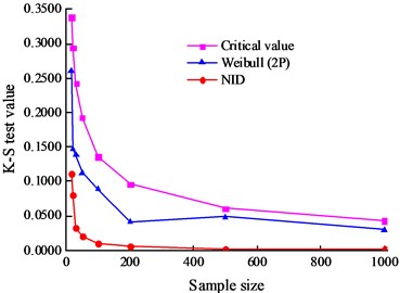
a) Sample 1#

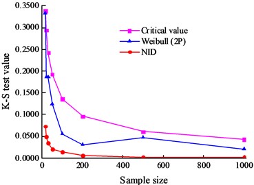
b) Sample 2#

The change in the chi-square test results with an increase in the sample size are shown in Fig. 5 for the simulated samples. It can be seen that both the NID distribution and Weibull distribution have passed the chi-square test. However, the test results of the NID distribution are considerably lower than those of the Weibull distribution; the test results of the Weibull distribution are one to two orders of magnitude greater than those of the NID distribution. Thus, the goodness of fit of the NID distribution is superior to that of the Weibull distribution. Moreover, the test results of the NID distribution are much more stable than those of the Weibull distribution.

Fig. 5The chi-square test results of the simulated data with the sample size

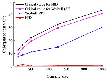
a) Sample 1#

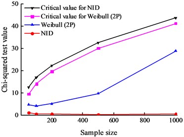
b) Sample 2#

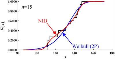
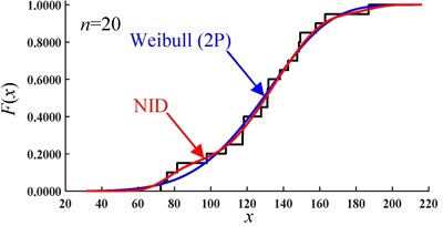
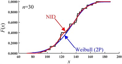
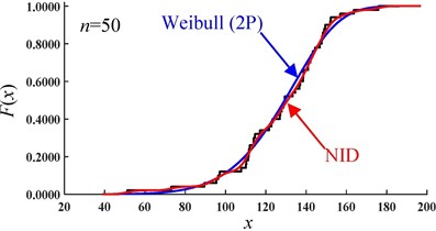
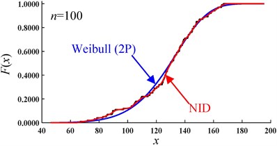
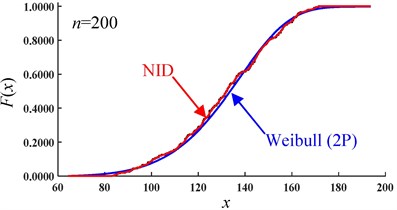
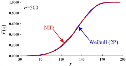
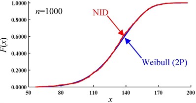
The CDF curves of the NID distribution and Weibull distribution for the simulated data of sample 1# are shown in Fig. 6. It is easy to see that, with an increase in the sample size, the CDF curves of the NID distribution are always closer to the empirical cumulative distribution function (EDF) curves than those of the Weibull distribution. Clearly, when the sample size is equal to 1000, the curves of the NID, Weibull and empirical distributions are nearly coincident.

Fig. 6Comparative CDF curves of the simulated data of sample 1# (sample size n)

a)

b)

c)

d)

e)

f)

g)

h)

The CDF values for simulated samples 1# and 2# with different sizes are shown in Tables 7 and 8, and the trends of the CDF values with sample size are shown in Fig. 7. Clearly, with an increase in the sample size, the cumulative probability values of the NID distribution are always equal to 1.0000 and are completely unaffected by the sample size. However, the cumulative probability values of the Weibull distribution are generally less than 1.0000, and there is a considerable amount of volatility when the sample size increases. It is evident from the above analysis that the NID distribution has a higher fitting precision and wider applicability.

Fig. 7Cumulative probability values of the simulated data with the sample size

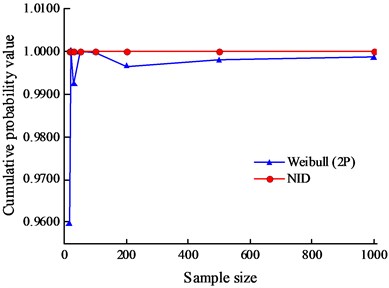
a) Sample 1#

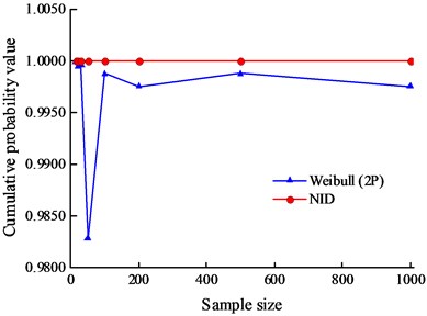
b) Sample 2#

6. Discussion

In the truncated interval, the cumulative probability values of classical distributions are usually less than 1.0000. To solve this problem, the normalization of the truncated classical distribution was introduced. The basic principle of normalized distribution is introduced as follows:

where $\tilde{f}\left(x\right)$ is the normalized PDF, $F\left(x\right)$ is the cumulative PDF, $f\left(x\right)$ is the classical PDF, $x$ is the value of the sample, and $R$ and $L$ are the maximum and minimum values of the sample, respectively.

The K-S test values of the normalized Weibull distribution for a 95 % confidence level are shown in Table 10. The sequence of the K-S test value of actual sample 1# is 0.0683 (NID) < 0.0969 (Weibull) < 0.1046 (normalized Weibull) < 0.3100 (Critical value). The sequence of the K-S test value of actual sample 2# is 0.0576 (NID) < 0.1475 (normalized Weibull) < 0.1495 (Weibull) < 0.2420 (Critical value). It can be found that all of the K-S test values pass the testing. However, all of the K-S test values of the normalized Weibull distribution are much more than those of the NID distribution, which indicates that the fitting ability of NID distribution is better than that of normalized Weibull distribution.

7. Conclusions

To accurately approximate the PDFs for geotechnical parameters, the NID method was introduced; several conclusions of this study are given below.

1) The PDFs of two sets of geotechnical samples were fitted with the NID distribution and Weibull distribution. The results show that, for the K-S test results, the chi-square test results and the cumulative probability values, the NID distribution is more accurate than the Weibull distribution. In addition, compared with the PDF curves of the Weibull distribution, those of the NID distribution can overcome the single-peak feature of the classical distributions and agree more closely with those of the actual distribution.

2) The effect of the sample size on the fitting accuracy for the NID distribution and Weibull distribution was investigated with the MC method, and eight simulated samples were produced. It can be found that with an increase in the sample size, the K-S test results of the NID distribution are all lower than those of the Weibull distribution. In addition, its convergence speed and stability are superior to those of the Weibull distribution. The cumulative probability values of the NID distribution are always equal to 1.0000 in the truncated interval and are unaffected by the sample size. However, the cumulative probability values of the Weibull distribution are generally less than 1.0000 and are unstable.

3) The comparison of the fitting accuracy between the NID distribution and the normalized Weibull distribution was also discussed, and the results show that, even if the cumulative probability values are equal to 1 for those two distributions, the fitting accuracy of the NID distribution is still higher than that of normalized Weibull distribution.