Study on unsteady aerodynamic characteristics of two trains passing by each other in the open air

Chen, Ye-gang; Wu, Qian

doi:10.21595/jve.2018.18695

Journal of Vibroengineering

Browse Journal

Submit article

Published: 31 March 2018

Check for updates

Study on unsteady aerodynamic characteristics of two trains passing by each other in the open air

Ye-gang Chen¹

Qian Wu²

^{1, 2}School of Computer Engineering, Yangtze Normal University, Chongqing, China

²Konkuk University, Seoul, Korea

Corresponding Author:

Ye-gang Chen

Cite the article Download PDF

Downloads 1560

WoS Core Citations 10

CrossRef Citations 6

Abstract

Based on three-dimensional, non-steady, compressive and unsteady control equations and $k - ε$ turbulence model, the paper adopts the finite volume method and moving grid technologies to conduct a numerical simulation analysis on pressure waves and aerodynamic forces (force moments) of two meeting trains in the open air. The simulation model has been validated by experimental test. Computational results show that during the meeting, the damage of the lateral window glass during the meeting is caused by that the window glass will be sucked out by negative pressures rather than be hit by positive pressures; both head wave pressure amplitude and tail wave pressure amplitude are in direct ratios to the square of the running speed; resistance values of the head and tail train experienced several changes, but the changing rules of the head train are opposed to those of the tail train; the lift force of the head train is downward all the time, the lift force is more than that of other train bodies, and lift force directions of the middle train and the tail train change alternately; the head train has the largest lateral force, the tail train ranks the second position, and the middle train ranks the last position; each train experiences 6 shaking force moment impacts including outward, inward, outward, inward, outward and inward impacts in succession; each train experiences 6 nodding force moment impacts, including downward, upward, downward, upward, downward and upward impacts, in succession.

1. Introduction

When high-speed trains are passing by each other, air fluctuation will be caused. At the instant when the head train and tail train are meeting, seriously instant changes will be generated to pressures on the head, the tail and meeting sides of trains [1]. Safety and comfort of running will be affected seriously by the meeting [2]. For example, trains will get obvious deformation; air inlet devices of the air conditioning system will be damaged; instant yaw of trains will be excessive [3, 4]. During the meeting, due to influential factors including impacts from aerodynamic forces and track unevenness, relative displacement, velocities and accelerations will be generated between parts and components of trains, where passengers’ riding comfort will be directly affected by the train vibration. In case of that trains are running at a high speed, effects caused by the meeting cannot be neglected. At present, pressure waves caused by the meeting are already deemed as an important index of assessing running safety.

Regarding aerodynamics of the meeting, some scholars have made a lot of experimental tests. Experimental methods mainly included full-scale real train tests and scaled model tests, where scaled model tests included wind tunnel tests and water tunnel tests. In a water tunnel, Wang and He [5, 6] studied scaled 1/25 train models of three kinds of head types in details, as well as pressure waves of the meeting under different track distances, and obtained experimental results which were consistent with full-scale real train tests. In order to assess the train design, Li [7] conducted real train tests of the meeting pressure waves with the linear interval of 5.1m, and obtained the pressure waves caused by passing trains with a high speed. Krajnović [8] conducted scaled model tests aiming at aerodynamic force of a high-speed train during its running in cross winds, and compared the experimental results with the wind tunnel tests. Xiong [9] conducted real train tests on the meeting pressure waves. Results show that the maximum amplitude of the meeting pressure waves on the train surface is 1195 Pa, and the running safety will not be affected under the linear interval of 4.4 m. Results of the full-scale real train tests can avoid impacts of the scale, and experimental data is relatively accurate. However, the cost is very high, needed time is long and the test will be affected by the environmental wind easily. Considering these problems in real train tests, researches on the meeting aerodynamics are mainly conducted on the experimental equipment with a scaled model. In a scaled model test, flowing conditions can be controlled under some cases, but problems about whether the scaled ratio is proper and how to simulate important impacts caused by ground and tracks in the wind tunnel and water tunnel tests should be also taken into account, while the experimental time is relatively long as well.

With the rapid development of computer technologies and algorithms, the meeting aerodynamics of trains can be studied through numerical simulation. Compared with traditionally experimental test, the numerical simulation method can give the required parameters at any time for simulation computation and can select optimum design according to computation results, so that human effort and materials can be saved and product design duration can be shortened. Tian [10, 11] conducted the numerical simulation on the meeting pressure waves of high-speed trains, studied influential factors of the meeting pressure waves, found the direct proportion relations between the meeting pressure waves and squares of meeting speeds, and analyzed impacts of the meeting pressure waves on bodies and lateral windows of trains. Bai [12] used the numerical simulation method to study the meeting pressure waves of high-speed maglev trains. Li [13] applied simulation technologies combining fluid software FLUENT with dynamics software SIMPACK to simulate the high-speed train meeting in an environment without crosswinds, and analyzed aerodynamic performance and dynamic features in the meeting. Through combining numerical simulation with a dynamic pressure system, Carassale [3] studied the meeting pressure waves of two trains which ran on a track at the speed of 200 km/h. Zhao [14] used the commercial software FLUENT to simulate two meeting trains in crosswind environment, and conducted a detailed analysis on aerodynamic performance of high-speed trains. Li [15] used the computational fluid dynamic method to study impacts of the train meeting on lateral windows and proposed a method for assessing the lateral window strength. However, these reported researches simplify the train model seriously, where trains are simplified into a smooth cylinder or two-dimensional models, and the correctness of the computational models is not verified by experimental test. Moreover, a moment balance equation of trains on tracks is established according to a static equation, and impacts of track unevenness are not taken into account.

Aiming at these problems, the paper studies the meeting aerodynamic characteristics and lateral window pressure waves of high-speed trains in the open air using advanced numerical simulation technologies. In this paper, impacts of track unevenness are considered, and the correctness of the computational model is verified by experiments. In this way, computational methods and basis are provided for strength design of lateral windows and running safety of the meeting high-speed trains in the open air.

2. Mathematical model of two meeting trains in the open air

Two meeting trains in the open air will form a three-dimensional, compressible, viscous and unsteady turbulent flow field. The differential equation in the form of Reynolds-averaged Navier-Stokes equations (RANS) [16, 17] is as follows.

Continuous equations:

1

\frac{d ρ}{d t} + \frac{\partial (ρ u)}{\partial x} + \frac{\partial (ρ v)}{\partial y} + \frac{\partial (ρ w)}{\partial z} = 0 .

Momentum conservation equations:

2

\begin{array}{l} \frac{\partial (ρ u)}{\partial t} + d i v (ρ u \vec{u}) = d i v (μ \cdot g r a d u) - \frac{\partial p}{\partial x} + S_{M x}, \\ \frac{\partial (ρ v)}{\partial t} + d i v (ρ v \vec{v}) = d i v (μ \cdot g r a d v) - \frac{\partial p}{\partial y} + S_{M y}, \\ \frac{\partial (ρ w)}{\partial t} + d i v (ρ w \vec{w}) = d i v (μ \cdot g r a d w) - \frac{\partial p}{\partial z} + S_{M z} . \end{array}

Energy conservation equations:

3

\frac{\partial (ρ i)}{\partial t} + d i v (ρ i \vec{u}) = d i v [(\frac{κ}{c_{p}} + \frac{μ_{t}}{σ_{T}}) g r a d T] + Φ .

Turbulence energy equations:

4

\frac{\partial (ρ k)}{\partial t} + d i v (ρ k \vec{u}) = d i v [(μ + \frac{μ_{t}}{σ_{k}}) g r a d k] - ρ ε + μ_{t} P_{G} .

Turbulence energy dissipation equation:

5

\frac{\partial (ρ ε)}{\partial t} + d i v (ρ ε \vec{u}) = d i v [(μ + \frac{μ_{t}}{σ_{ε}}) g r a d ε] - ρ C_{2} \frac{ε^{2}}{k} + μ_{t} C_{1} \frac{ε}{k} P_{G},

6

μ_{t} = ρ C_{μ} \frac{k^{2}}{ε},

7

P_{G} = 2 [{(\frac{\partial u}{\partial x})}^{2} + {(\frac{\partial v}{\partial y})}^{2} + {(\frac{\partial w}{\partial z})}^{2}] + {(\frac{\partial u}{\partial y} + \frac{\partial v}{\partial x})}^{2} + {(\frac{\partial u}{\partial z} + \frac{\partial w}{\partial x})}^{2} + {(\frac{\partial v}{\partial z} + \frac{\partial w}{\partial y})}^{2}

+ λ (d i v \vec{u}) .

where: $u$ , $v$ , $w$ are components of flow velocity in $x$ , $y$ and $z$ coordinate directions, $ρ$ is fluid density, $μ$ is fluid dynamic viscosity density, $μ_{t}$ is turbulence viscosity, $k$ is turbulence kinetic energy, $ε$ is turbulence kinetic energy dissipation efficiency, $T$ is fluid temperature, $κ$ is air thermal conductivity, $c_{p}$ is specific heat of air mass at constant pressure, $C_{1}$ , $C_{2}$ , $C_{μ}$ , $σ_{k}$ , $σ_{ε}$ are constants, and empirical values are set as 1.44, 1.92, 0.09, 1.0 and 1.3, $Φ$ is dissipation function, $S_{M x}$ , $S_{M y}$ , $S_{M z}$ are source items of momentum equations in $x$ , $y$ , $z$ directions:

8

S_{M x} = [\frac{\partial}{\partial x} (μ \frac{\partial u}{\partial x}) + \frac{\partial}{\partial y} (μ \frac{\partial v}{\partial x}) + \frac{\partial}{\partial z} (μ \frac{\partial w}{\partial x})] + \frac{\partial}{\partial x} (λ d i v \vec{u}),

9

S_{M y} = [\frac{\partial}{\partial x} (μ \frac{\partial u}{\partial y}) + \frac{\partial}{\partial y} (μ \frac{\partial v}{\partial y}) + \frac{\partial}{\partial z} (μ \frac{\partial w}{\partial y})] + \frac{\partial}{\partial y} (λ d i v \vec{u}),

10

S_{M z} = [\frac{\partial}{\partial x} (μ \frac{\partial u}{\partial z}) + \frac{\partial}{\partial y} (μ \frac{\partial v}{\partial z}) + \frac{\partial}{\partial z} (μ \frac{\partial w}{\partial z})] + \frac{\partial}{\partial z} (λ d i v \vec{u}) .

In a RNG $k$ - $ε$ model [18, 19] (Renormalization Group, RNG), impacts of a small scale are embodied by the viscosity item obtained after large-scale motion and correction, so the small-scale motion can be removed from the controllable equation systematically. Through correcting turbulence viscosity and considering the rotation in average flow, the time-average strain rate of main flows can be reflected. Obviously, the RNG $k$ - $ε$ model can effectively deal with flows with a high strain rate and high-degree of streamline bending. In addition, during computing the high-speed train meeting, it is steadier and can get converged more easily compared with the standard $k$ - $ε$ model. Therefore, it is widely applied in engineering practice. Finally, the RNG $k$ - $ε$ turbulence model is selected in unsteady computation of two meeting trains.

3. Numerical model of two meeting trains in the open air

3.1. Geometric model and computational domain

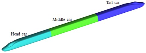
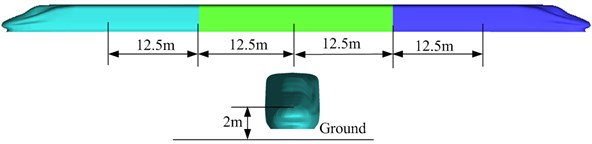
High-speed train is a complicated, thin and long structure. Computational amount will be very large if the numerical simulation is conducted on flow field of the complete train. The middle flow field structure of trains is basically steady because the middle structure has some distance from the head train. The paper adopts a train model including head-middle-tail trains, where the head train and the tail train have the same shape. Meanwhile, in order to avoid redundancy grids, the train was simplified into a geometric body composed of smooth curved faces, as shown in Fig. 1.

Fig. 1Geometric model of the high-speed train

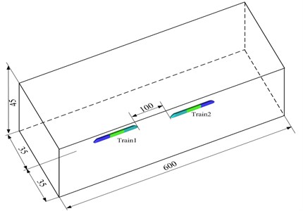
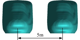
When a computational domain of two meeting trains is established, the sizes of the computational domain should be big enough with considering full development of the flow field as well as impacts of air flows. Theoretically, the computational domain of the flow field around the high-speed train should be infinitely large. However, only limited space can be adopted in the actual numerical simulation. On the premise that flowing of fluids around the high-speed train is not affected, a proper computational domain should be selected, namely boundaries of the computational domain should be far enough from the high-speed train surface, and thus high-speed air flows generated from the high-speed train running only have very small impacts on boundary regions. However, the larger computational domain will lead to the larger amount of meshes, which will reduce the computational speed. In order to guarantee the computational accuracy and increase the computational speed at the same time, multiple computational domains were established for comparison. Finally, a properly computational domain was selected, as shown in Fig. 2. Length, width and height of the computational domain are 600 m, 70 m and 45 m, respectively; distance between the train and the ground is 0.25 m; train head distance of high-speed trains is 100 m during the meeting; track distance is 5 m, as shown in Fig. 3.

Fig. 2Computational domain of two meeting trains in the open air

3.2. Grid generation

Grid division and quality are very important for the computational efficiency, convergence and accuracy. In the computational space domain, grids with big sizes were adopted. Grid refinement was conducted on regions with big flow field changes. The scheme of layer-by-layer transition was used from fine grids to rough grids. Rational amount of boundary layers was used, so that the size of boundary layers could be slowly changed to the size of main body grids. Grids on the first boundary layer were 0.2 mm thick. In order to realize the smooth connection with grids outside the near wall face region and ensure grid quality, grids with 6 boundary layers were set with the growth ratio of 2.5. As a result, the accuracy of applied wall face functions in the near wall face region can be ensured. Grids in regions such as tail flows and train surface which affect the flow field obviously were refined. Flow fields were smoother at the positions far from the train, so spatial grids far from the train region were larger. Finally, the amount of grids is reduced, while the computational accuracy will not be reduced.

Fig. 3Track distance of two meeting trains in the open air

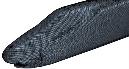
In general, if the computational result deviation of two sets of grids is lower than 2 %, the computational results will be deemed to be unrelated with the grids. Regarding model in this paper, three sets of grids were adopted for trial computation, respectively. Results are shown in Table 1. Amounts of computational grids are 14.15 million, 17.89 million and 19.72 million, respectively. Results show that the computational error is smaller than 1.92 % when the total amount of grids is more than 19.72 million. Therefore, the grid amount of the computational model proposed in this paper is controlled over 19.72 million. In other words, experimental requirements for grid independence can be satisfied when the maximum size in the train external field is 1500 mm, and the maximum size of the train surface is 90 mm. Tetrahedral grids are used for dividing grids of the computational domain. Local grids of the high-speed train are shown in Fig. 4.

Table 1Verification of mesh independence

Grid scheme	External-field maximum grid / mm	Maximum grid of train / mm	Total amount of grids (x10,000)	Grid increment	Pressure value of monitoring point / Pa	Relative change
Scheme 1	3000	120	1415		–678.5
Scheme 2	2000	100	1789	26.43 %	–710.7	4.75 %
Scheme 3	1500	90	1972	10.23 %	–724.4	1.92 %

Fig. 4Local grids of the high-speed train

3.3. Boundary conditions

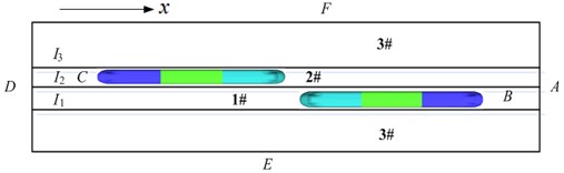
Two meeting trains are defined as an observed train and a passing train. In order to simulate relative motion between trains and the open air, the computational flow field was divided into 3 regions. Region 1# refers to regions around the passing train and regions in front of and behind the advancing direction. Region 2# refers to regions around the observed train and regions in front of and behind the advancing direction. Region 3# refers to regions around the open air, inlet and outlet. Fig. 5 shows flow field partition diagram of two meeting trains in the open air.

Numerical simulation of the external flow field of high-speed trains was conducted in a finite region. Therefore, proper boundary conditions should be defined on region boundaries. Whether boundaries conditions could be established correctly directly affects correctness and computational accuracy of the numerical computation. It has a clear physical significance to confirm that boundary condition requirements could satisfy mathematical appropriateness. In flow field computation in the paper: end faces A and D are pressure boundary conditions; train body surfaces B and C of two trains are wall faces without slippage, the running speeds are given in the $x$ direction, and speeds in $y$ and $z$ directions are 0; open regions E and F outside entrance and exit of the external flow field are set as symmetric far-field boundary conditions; regional boundaries $I_{1}$ , $I_{2}$ and $I_{3}$ are set as slippage boundary conditions; as for intersected interfaces, the “interface pair” was used to process movable parts and stationary parts. The boundary condition of “without slippage wall face” was given to other surfaces including the ground. A standard wall face function was used for approximate simulation of turbulent flow field around the wall faces.

Fig. 5Flow field partition of two meeting trains in the open air

3.4. Moving grid technologies

The fluid software FLUENT is used in the numerical simulation. It contains moving grid technologies which are used to solve relative motion of objects. In flow field partition, as for two parts with relative motion, such as a fixed part and a moving part, the interface face among them is connected by a slippage interface. Two flow fields can exchange information by the interface. The interface is set as a slippage boundary condition.

Fig. 6Relations between grid increase, deletion and train motion

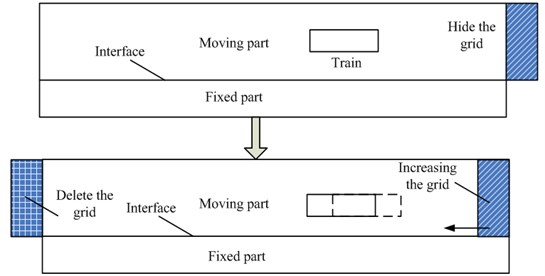
In order to achieve numerical simulation of train motion, the moving grid method shall be adopted, where the whole layer of grids will be added and deleted, and moving grid update is conducted on nodes in a computational domain. Fig. 6 displays relations between grid increase, deletion and train motion. In Fig. 6, a layer of grids is defined. In order to ensure invariability of computational amount of the complete flow field, it is firmly set as hidden grids and does not take part in the computation. When the train moves by a certain distance, the layer of hidden grids will be added to the movable flow field; a layer of grids on the left side of the movable flow field will be deleted; and then, all the nodes in the movable flow field will move leftwards at the train speed. In this way, train motion can be achieved, and computational domains and computational amount of the complete flow field can be kept unchanged.

3.5. Experimental validation on the numerical model

The computational model of aerodynamic characteristics for two meeting trains is very complicated, so its correctness should be verified by experiments. As shown in Fig. 7, a tested point was arranged on the window at the train nose tip to measure the meeting pressure waves of two trains. The high-speed trains ran at the speed of 300 km/h, and the environmental wind speed was very small, so that impacts on experimental results were avoided. Selection of sensors should obey principles of high accuracy and small impacts on flow fields. Therefore, in the experiment, a piezoresistive sensor produced by ENDEVCO Company was selected [20-24]. With a small size, the sensor was only 0.76 mm thick, bringing a small impact on the flow. The sensor was installed easily. In the experiment, the sensor was directly adhered by double sided adhesive tapes on the train surface. Data measured by the sensor was transmitted to a computer by a data collector. In the experimental test, the collected data should be filtered to remove the interference signal [25-29]. Finally, through processing the data, the meeting pressure waves of two trains could be obtained, as shown in Fig. 8.

Fig. 7Tested points of the meeting pressure waves of two high-speed trains

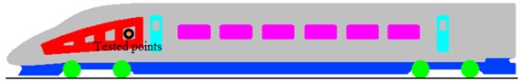
Fig. 8The meeting pressure waves of two high-speed trains

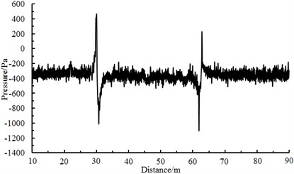
It is shown in Fig. 8 that two obvious peak values and valley values are in the meeting pressure waves, where the first peak value and valley value reflect the meeting process between the observed head train and the passing head train, while the second peak value and valley value reflect the meeting process between the observed tail train and the passing tail train. Similarly, the numerical computation model and boundary conditions were used to simulate the meeting pressure waves of two trains at the same speed. Head waves and tail waves of two meeting trains were computed and compared with experimental results, as shown in Table 2. It is shown in Table 2 that when the running speed is 300 km/h, the tested head wave amplitude is 1501 Pa, the computational value is 1456 Pa, and the relative error is –3.00 %; the tested tail wave amplitude is 1329 Pa, the computational value is 1368 Pa, and the relative error is 2.93 %; when the running speed is 350 km/h, the relative errors of head waves and tail waves between experimental and numerical simulation are –4.38 % and –3.87 %, respectively. Errors are attributed to differences between the computational model and real trains, and tested results are also affected by local weather conditions to a certain extent. In addition, the deviation is also between positions of tested points and points on the numerical computation model. However, as a whole, the absolute values of errors between tested data and computational data are smaller than 5 %. Obviously, the numerical computation is feasible and can approximately reflect the meeting pressure wave of two trains.

Table 2Comparisons of the meeting pressure waves between experiment and simulation

Parameters	Running speed = 300 km/h		Running speed = 350 km/h
Parameters	Head waves	Tail waves	Head waves	Tail waves
Experimental values	1501 Pa	1329 Pa	2077 Pa	1965 Pa
Computational values	1456 Pa	1368 Pa	1986 Pa	1889 Pa
Relative errors	–3.00 %	2.93 %	–4.38 %	–3.87 %

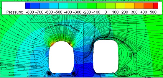
Fig. 9Pressure contours of two meeting trains in the open air

a) Before two train meeting

b) During two train meeting

c) After two train meeting

4. Flow field characteristics of two meeting trains in the open air

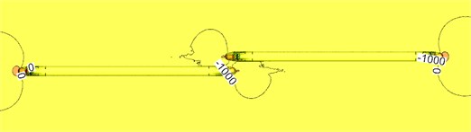
Fig. 9 shows a pressure distribution contour of two meeting trains with 350 km/h on the flat ground. Fig. 10 shows train surface pressure contour during two train meeting. It is shown in Fig. 9 and Fig. 10 that when the high-speed train is meeting, pressures distributed on the meeting side will be more than those on the side without meeting; a large region of negative pressures appeared on the side without meeting, the train top and bottom; a few of positive pressure regions appeared on the meeting side compared with the side without meeting. Obviously, damage of the lateral window glass during two train meeting is mainly caused by that the window glass will be sucked out by negative pressures rather than be damaged by positive pressure impact.

Fig. 10Pressure distribution of two meeting trains in the open air

5. Analysis on aerodynamic performance of two meeting trains in the open air

5.1. Arrangement of observed points of the meeting pressure waves

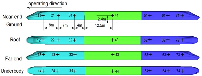
In order to find relations of the meeting pressure waves on the surfaces of high-speed trains in the open air, observed points at the same positions, as shown in Fig. 11, were extracted on head train, middle train and tail train of the observed train, where the observed points were 2.4 m high above the ground. Therein, observed points 11, 21, 31, 41, 51, 61 and 71 were near the wall face (meeting side); observed points 12, 22, 32, 42, 52, 62 and 72 were on the surface of train top center. Observed points 13, 23, 33, 43, 53, 63 and 73 were on the train surface far from the wall face (sides without the meeting). Observed points 14, 24, 34, 44, 54, 64 and 74 were on the surface of train bottom center. Detailed positions of observed points are shown in Fig. 11.

Fig. 11Arrangement of observed points on the train surface

5.2. Pressure wave characteristics in two meeting trains

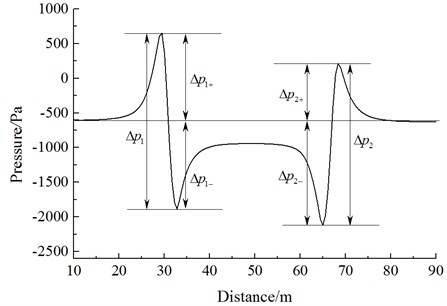
Fig. 12 shows a history curve of pressure changes at the lateral window of the meeting side (observed point 11). It is shown in Fig. 12:

(1) The air pressure wave intensity during the meeting is the amplitude of air pressure waves, which is also called as full wave and denoted by $Δ P$ . $Δ P_{1}$ is the full-wave amplitude of the head wave. $Δ P_{1 +}$ is the positive wave amplitude of the head wave. $Δ P_{1 -}$ is the negative amplitude of the head wave. $Δ P_{2}$ is the full-wave amplitude of the tail wave. $Δ P_{2 +}$ is the positive wave amplitude of the tail wave. $Δ P_{2 -}$ is the negative wave amplitude of the tail wave:

11

Δ P = \{\begin{array}{l} |Δ P_{+}| + |Δ P_{-}|, |Δ P_{+}| + |Δ P_{-}| \leq 0, \\ ||Δ P_{+}| - |Δ P_{-}||, |Δ P_{+}| + |Δ P_{-}| > 0 . \end{array}

(2) During the moment before arrival at observed point 11 of the observed train from the head of the passing train, the pressure already begins increasing and then increases rapidly. When the pressure passes the train nose and reaches the observed point, a positive-negative pulse is generated, namely the head wave. Constant-amplitude fluctuations began after occurrence of the maximum negative pulse. When the pressure passes the nose of tail train and passes the observed point, a negative-positive pulse is generated, namely the tail wave.

(3) During the meeting, the head wave of the air pressure full wave is more than the tail wave; absolute value of the negative wave is more than that of the positive wave. This phenomenon is more obviously on the tail train.

(4) The air pressure wave intensity in the meeting is a time gradient of the pressure wave, namely:

12

g r a d \nabla P = \frac{Δ P}{Δ t} .

(5) Pressure coefficient is defined as:

13

C_{p} = \frac{2 P}{ρ v^{2}},

where: $P$ is aerodynamic pressure, $ρ$ is air density, $v$ is running speed of trains.

Fig. 12Pressure changes at the lateral window during the meeting

5.3. Distributions of pressure waves of two meeting trains

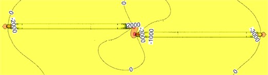
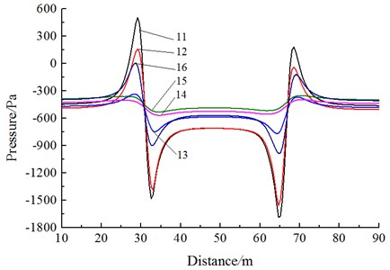
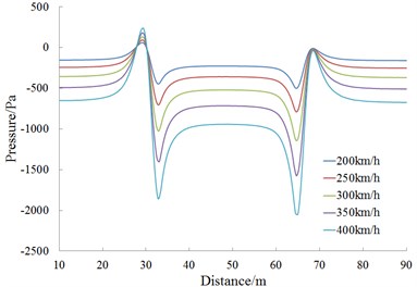
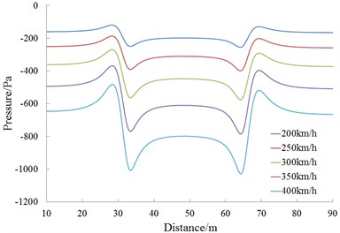
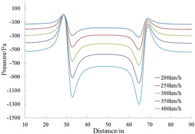
In order to study rules of pressure waves of cross section for two meeting trains, the history curves of pressure waves in observed points 11, 12, 13, 14, 15 and 16 were compared and analyzed. Fig. 13 shows pressure curves of different observed points on the cross section corresponding to the observed point 1 during the meeting. Through analyzing the Fig. 11, we can find:

(1) With the increased running speed, the pressure value increased obviously around positive waves of the head wave and the tail wave. The head wave $Δ P_{1 +}$ and the tail wave $Δ P_{2 +}$ near the wall face have positive pressure values. The head wave $Δ P_{1 -}$ and the tail wave $Δ P_{2 -}$ near the wall face of the train body have negative pressure values. In addition, $|Δ P_{1 -}| > |Δ P_{1 +}|,$ $|Δ P_{2 -}| > |Δ P_{2 +}|$ and $|Δ P_{1}| > |Δ P_{2}|$ are satisfied. Train top, bottom and the train body far from the wall face are located in negative pressure regions.

(2) Obviously, with the increased running speed, pressures at observed points 11, 12 and 16 are much more than pressures at other observed points, namely maximum pressures near the wall face (train meeting side) appear at the head wave and the tail wave; therein, the largest pressures appear at the observed point 11. Obviously, the positive wave amplitude is the largest at the nose height. From bottom to top, the positive wave amplitude of the train decreases gradually.

(3) On the train cross section, the positive wave amplitude of head waves at each observed point satisfies 11>12>16>13>15>14; the negative wave amplitude of head waves at each observed point satisfies 11>12>16>13>15>14; tail waves present the same rules at each observed point; negative wave amplitudes are more than positive wave amplitudes.

(4) As for positive waves, the head wave tends to decrease along the running direction during the meeting. The tail wave shows the opposite phenomenon. Along the running direction, the positive waves tend to increase. Along the running direction, positive waves of the head wave decrease from 475.45 Pa to 378.95 Pa; positive waves of the tail wave increase from 297.89 Pa to 375.12 Pa.

(5) As for negative waves, the head wave tends to increase along the running direction during the meeting. The tail wave shows the opposite phenomenon and tends to decrease along the running direction; along the running direction, the negative waves of the head wave increase from 479.56 Pa to 618.25 Pa, and negative waves of the tail wave decrease from 595.21 Pa to 464.44 Pa.

(6) As for the full wave, during the meeting, the head waves decrease firstly and then increase along the running direction; full-wave amplitudes of the tail wave tend to decrease along the running direction.

Fig. 13Pressure curves of different observed points during the meeting

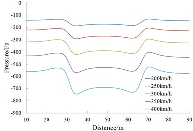
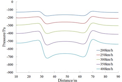
5.4. Change rules of pressure waves during the meeting

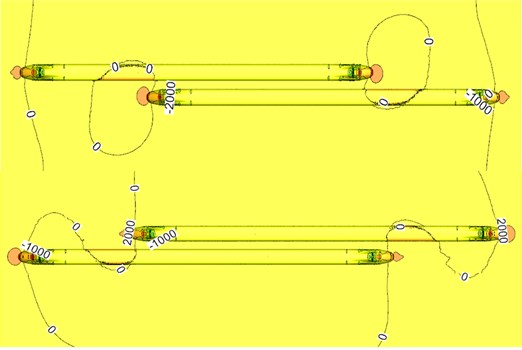
Fig. 14 shows a pressure curve of the cross section on observed point 1 during the meeting. According to Fig. 14, pressures of observed points 11, 12, 13, 14, 15 and 16 are analyzed, as follows:

(1) When the train head of Train 1 passes observed points arranged around the lateral window of Train 2 (such as observed points 11, 12, 14 and 15), a pressure wave peak value is caused firstly, and then the pressure sharply decreases to a valley value; when the train tail passes the observed point, a valley value is caused firstly and then the pressure increases sharply to a peak value.

(2) History curves of pressures at observed points show that when the train head is meeting, aerodynamic effects are more than aerodynamic effects when the train tail is passing by each other.

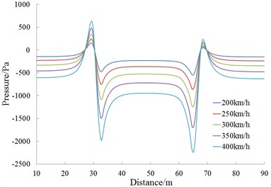
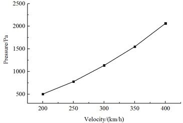
Fig. 15 is the change curve of the head wave amplitude at the observed point 11 during the meeting. It is shown in Fig. 15 that; the head wave pressure amplitudes are in direct ratio to the square of running speed during the meeting.

Fig. 14History curves of pressures at different observed points under different speeds

a) Observed point 11

b) Observed point 12

c) Observed point 13

d) Observed point 14

e) Observed point 15

f) Observed point 16

Fig. 15Change curve of head wave amplitudes with different running speeds

5.5. Analysis on aerodynamic action forces of two meeting trains

Computational coordinates of aerodynamic action forces during the meeting are shown in Fig. 16(a), where $F_{x}$ is the resistance; $F_{y}$ is the lateral force; $F_{z}$ is the lift force; $M_{x}$ is the lateral rolling force moment; $M_{y}$ is the nodding force moment; $M_{z}$ is the shaking force moment. Extraction of aerodynamic forces is obtained through applying region integral method to the outer surface. Simplified centers of aerodynamic forces and aerodynamic force moments in this paper are shown in Fig. 16(b).

Fig. 16Schematic diagram of aerodynamic force moments

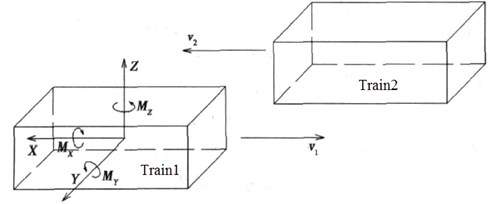
a) Coordinate relations of aerodynamic force moments

b) Positions of aerodynamic force moments

Fig. 17 shows the change curve of the resistance with the running speed on Train 2 during the meeting. It is shown in Fig. 17:

(1) Along the running direction, resistance values on each train of Train 2 are positive. Obviously, the resistance direction is opposite to the running direction; the head train and the tail train exerted the largest effects; resistance values of the middle train gradually decrease with the increased meeting distance; resistance values of the middle train don’t change obviously during the meeting.

(2) With the increased running speed, resistance values of each train increase, where resistance values caused by the passing head train have the largest effects.

(3) When the train head of Train 1 is passing Train 2, the head train resistance of Train 2 generates a peak value at first, and then the resistance sharply increases and decreases to a peak value and valley value, respectively; when the train tail of Train 1 is passing the head train of Train 2, a peak and valley value is generated at first, and then the resistance sharply decreases/increases to a peak-to-peak value. Resistance distributions of the tail train for Train 2 are opposite to those of the head train for Train 2. Resistance distributions of Train 1 are opposite to those of Train 2.

(4) During the meeting in the open air, resistance values of the head and tail train experienced several changes, but the changing rules of the head train are opposed to those of the tail train. When the nose of Train 1 begins meeting the nose of Train 2, the stagnation pressure on nose tip of head train for Train 2 also increases correspondingly due to effects of nose positive pressure regions of Train 1, so resistance values of the complete head train increase; when nose of Train 1 is located on the lateral face of Train 2, the stagnation pressure of the nose of Train 2 decreases due to effects of negative pressure regions on the surface of train bodies of Train 1, so resistance values of the complete head train decrease. When the head train of Train 1 is passing the tail train of Train 2, due to effects of positive and negative pressure regions on the nose of tail train for Train 1, the resistance will change in the resistance decrease-resistance increase form, and then resistance states are recovered in the open air.

Fig. 17Change curves of resistance values on each train body

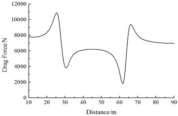
a) Resistance values of the head train

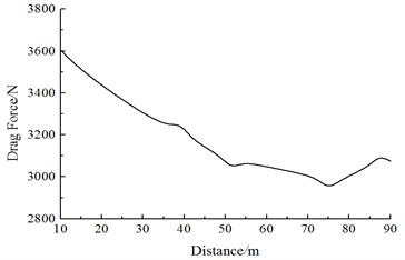
b) Resistance values of the middle train

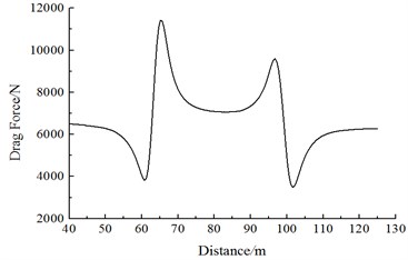
c) Resistance values of the tail train

Fig. 18Change curves od lift forces on each train body

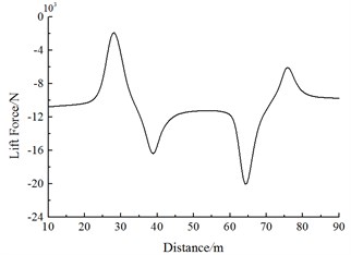
a) Lift forces of the head train

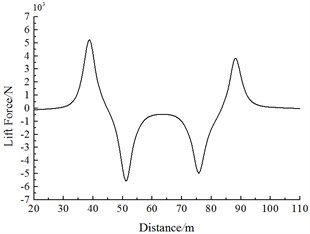
b) Lift forces of the middle train

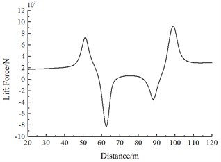
c) Lift forces of the tail train

Fig. 18 shows the change curve of the lift force on Train 2 during the meeting. It is shown in Fig. 18:

(1) Along the running direction, lift force values of head trains for Train 1 and Train 2 are negative. With the increased running speeds, lift forces of each train body increase. Lift force values caused by head trains of each train exerted the largest effects. With regard to lift force of the head train, lift force amplitudes of the tail wave are more than those of the head wave.

(2) When the head train of Train 1 is passing Train 2, a positive lift force peak value is firstly generated at the middle train and tail train of Train 2. Then, the lift force sharply decreases to a negative valley value. When the train tail of Train 1 is passing the head train of Train 2, a negative valley value of lift forces is caused firstly, and then the lift force sharply increases to a positive peak value. Lift force amplitudes of head wave lift force for the middle and the tail trains are more than those of the tail wave.

Fig. 19 shows the change curve of the lateral force on the head train of Train 2 during the meeting. It is shown in Fig. 19 that:

(1) With the increased running speed, the lateral force on each train body increases. Lateral force values caused by the head train and tail train on each train exerted the largest effects. The first wave lateral force peak of the head wave in the head train is more than the amplitude of the second wave lateral force of the head wave.

(2) When the train head of Train 1 is passing Train 2, the head train, middle train and tail train of Train 2 generated a positive peak value at first, and then the lateral force sharply decreases to a negative valley value; when the tail of Train 1 is passing the head train of Train 2, Train 2 generates a negative valley value at first, and then the lateral force sharply increases to a positive peak value.

Fig. 19Change curve of the lateral force on the head train

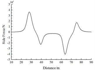
Fig. 20 shows the change curve of aerodynamic force moment on head train of Train 2 during two trains meeting. It is shown in Fig. 20 that:

(1) When the train head of Train 1 is passing Train 2, the head train, middle train and tail train of Train 2 generate a positive lateral rolling force moment peak value at first, and then the lift force sharply decreases to a negative valley value; when the train tail of Train 1 is passing the head train of Train 2, the Train 2 generates a negative valley value at first, and then the lateral rolling force moment sharply increases to a positive peak value.

(2) When the train head or train tail of Train 1 is passing Train 2, shaking force moments of Train 1 and Train 2 present three peak values. The head train, middle train and tail train of Train 2 generate a positive shaking force moment peak value at first, then the shaking force moment sharply decreases to the negative valley value when the train head of the passing train has passed 1/4 train length, and a positive peak value in the opposite direction is also experienced; when the train tail of Train 1 is passing the head train of Train 2, the Train 2 generates a negative valley value at first, then the shaking force moment sharply increases to a positive peak value, and next the shaking force moment sharply decreases to a negative valley value. Shaking force moments of the complete train body experienced 6 direction changes. Obviously, during the meeting, each train body experienced 6 impact force moments, including outward, inward, outward, inward, outward and inward impact force moments, in succession.

(3) When the train head or train tail of Train 1 is passing Train 2, the nodding force moments of Train 2 present three peak values. The head train of Train 1 generates a positive nodding force moment peak value at first, then the nodding force moment sharply decreases to a negative valley value when the train head of the passing train has passed 1/4 train length, and a positive peak value in the opposite direction is experienced; when the train tail of Train 1 is passing the train tail of Train 2, Train 1 generates a negative valley value at first, then the nodding force moment sharply increases to a positive peak value, and next the nodding force moment sharply decreases to a negative valley value. Nodding force moments of the head train of Train 1 are negative, while the distribution rules are the same with those of the middle train and tail train. When Train 1 is passing Train 2, the nodding force moment distribution rules of Train 2 are similar to those of nodding force moments of the passing train, where the values are equal, but the directions are opposite. Nodding force moments of the complete train body experience 6 direction changes. Obviously, during the meeting, each train experiences 6 impact force moments, including downward, upward, downward, upward, downward and upward impact force moments, in succession.

Fig. 20Change curves of force moments on the head train

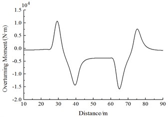
a) Lateral rolling force moments

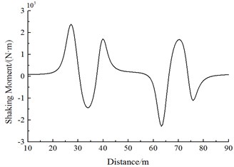
b) Shaking force moments

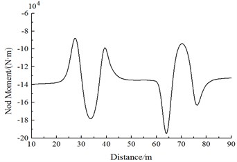
c) Nodding force moments

6. Conclusions

Based on three-dimensional, non-steady, compressive and unsteady control equations and $k$ - $ε$ turbulence model, the paper adopts the finite volume method and moving grid technologies to conduct a numerical simulation analysis on pressure waves and aerodynamic forces (force moments) of two meeting trains in the open air. The following conclusions are obtained:

1) During the meeting, pressures on the meeting side will be more than those on another side; a large region with negative pressures appears on the side without the meeting, the train top and bottom; a few of positive pressure regions appears on the meeting side compared with another side. Obviously, the damage of the lateral window glass during the meeting is caused by that the window glass will be sucked out by negative pressures rather than be hit by positive pressures.

2) During the meeting, the train head of Train 1 always generates a pressure wave peak value when passing each observed point, and then the pressure sharply decreases to a valley value; when the train tail of Train 1 is passing the observed point, a pressure wave valley value is caused at first, and then the pressure sharply increases to a peak value. Both head wave pressure amplitude and tail wave pressure amplitude are in direct ratios to the square of the running speed during the meeting.

3) During the meeting in the open air, resistance values of the head and tail train experienced several changes, but the changing rules of the head train are opposed to those of the tail train. During the meeting, the lift force of the head train is downward all the time, the lift force is more than that of other trains, and lift force directions of the middle train and the tail train change alternately; during the meeting, the head train has the largest lateral force, the tail train ranks the second position, and the middle train ranks the last position.

4) During the meeting, the shaking force moments of the complete train experience 6 directional changes, where each train experiences 6 impact force moments, including outward, inward, outward, inward, outward and inward impact force moments, in succession. Similarly, nodding force moments of the complete train experience 6 directional changes, where during the meeting, each train experiences 6 impact force moments, including downward, upward, downward, upward, downward and upward impact force moments, in succession.

References

Liu T., Zhang J. Effect of landform on aerodynamic performance of high-speed trains in cutting under cross wind. Journal of Central South University, Vol. 20, Issue 3, 2013, p. 830-836.

Publisher
Li Y., Hu P., Cai C. S., et al. Wind tunnel study of a sudden change of train wind loads due to the wind shielding effects of bridge towers and passing trains. Journal of Engineering Mechanics, Vol. 139, Issue 9, 2012, p. 1249-1259.

Publisher
Carassale L., Brunenghi M. M. Dynamic response of trackside structures due to the aerodynamic effects produced by passing trains. Journal of Wind Engineering and Industrial Aerodynamics, Vol. 123, 2013, p. 317-324.

Publisher
Zhao X. L., Sun Z. X. A new method for numerical simulation of two trains passing by each other at the same speed. Journal of Hydrodynamics, Series B, Vol. 22, Issue 5, 2010, p. 697-702.

Publisher
Wang Y. W., Yang G. W., Huang C. G., et al. Influence of tunnel length on the pressure wave generated by high-speed trains passing each other. Science China Technological Sciences, Vol. 55, Issue 1, 2012, p. 255-263.

Publisher
He X. H., Zou Y. F., Wang H. F., et al. Aerodynamic characteristics of a trailing rail vehicles on viaduct based on still wind tunnel experiments. Journal of Wind Engineering and Industrial Aerodynamics, Vol. 135, 2014, p. 22-33.

Publisher
Li M. S., Lei B., Lin G. B., et al. Field measurement of passing pressure and train induced ariflow speed on high speed maglev vehicles. Acta Aerodynamica Sinica, Vol. 24, Issue 2, 2006, p. 209-212.

Search CrossRef
Krajnović S., Ringqvist P., Nakade K., et al. Large eddy simulation of the flow around a simplified train moving through a crosswind flow. Journal of Wind Engineering and Industrial Aerodynamics, Vol. 110, 2012, p. 86-99.

Publisher
Xiong X. H., Liang X. F. Analysis of air pressure pulses in meeting of CRH2 EMU trains. Journal of the China Railway Society, Vol. 31, Issue 6, 2009, p. 15-20.

Search CrossRef
Tian H. Q., He D. X. 3-D numerical calculation of the air pressure pulse from two trains passing by each other. Journal of the China Railway Society, Vol. 24, Issue 3, 2001, p. 18-22.

Search CrossRef
Liang X. F., Tian H. Q. Test research on crossing air pressure pulse of 200km/h electric multiple unit. Journal of Central South University of Technology (Natural Science), Vol. 33, Issue 6, 2002, p. 621-624.

Search CrossRef
Bai H. Q., Lei B., Zhang W. H. Numerical study of the pressure load caused by high-speed passing maglev trains. Acta Aerodynamica Sinica, Vol. 24, Issue 2, 2006, p. 213-217.

Search CrossRef
Li R. X., Jing Z., Jie L. Influence of air pressure pulse on side windows of high-speed trains passing each other. Journal of Mechanical Engineering, Vol. 46, Issue 4, 2010, p. 87-92.

Publisher
Zhao Y., Zhang J., Li T., et al. Aerodynamic performances and vehicle dynamic response of high-speed trains passing each other. Journal of Modern Transportation, Vol. 20, Issue 1, 2012, p. 36-43.

Publisher
Li R. X., Liu J., Qi Z. D., Zhang W. H. Air pressure pulse developing regularity of high-speed trains crossing in open air. Journal of Mechanical Engineering, Vol. 47, Issue 4, 2011, p. 125-130.

Publisher
Chen J. H. Petascale direct numerical simulation of turbulent combustion-fundamental insights towards predictive models. Proceedings of the Combustion Institute, Vol. 33, Issue 1, 2011, p. 99-123.

Publisher
Bianco V., Manca O., Nardini S. Numerical investigation on nanofluids turbulent convection heat transfer inside a circular tube. International Journal of Thermal Sciences, Vol. 50, Issue 3, 2011, p. 341-349.

Publisher
Antonov N. V., Kapustin A. S. Effects of turbulent mixing on critical behaviour in the presence of compressibility: renormalization group analysis of two models. Journal of Physics A: Mathematical and Theoretical, Vol. 43, Issue 40, 2010, p. 405001-1.

Publisher
Kamyar A., Saidur R., Hasanuzzaman M. Application of computational fluid dynamics (CFD) for nanofluids. International Journal of Heat and Mass Transfer, Vol. 55, Issue 15, 2012, p. 4104-4115.

Publisher
Li J., Deng G., Luo C., et al. A hybrid path planning method in unmanned air/ground vehicle (UAV/UGV) cooperative systems. IEEE Transactions on Vehicular Technology, Vol. 65, Issue 12, 2016, p. 9585-9596.

Publisher
Li J., He S., Ming Z., et al. An intelligent wireless sensor networks system with multiple servers communication. International Journal of Distributed Sensor Networks, Vol. 11, 2015, p. 960173.

Search CrossRef
Wei W., Song H., Li W., et al. Gradient-driven parking navigation using a continuous information potential field based on wireless sensor network. Information Sciences, Vol. 408, 2017, p. 100-114.

Publisher
Li J., Zhang S., Yang L., et al. Accurate RFID localization algorithm with particle swarm optimization based on reference tags. Journal of Intelligent and Fuzzy Systems, Vol. 31, Issue 5, 2016, p. 2697-2706.

Publisher
Cui K., Zhao T. T. Unsaturated dynamic constitutive model under cyclic loading. Cluster Computing, Vol. 20, Issue 4, 2017, p. 2869-2879.

Publisher
Qiang, Mei, et al. X. Modified repetitive learning control with unidirectional control input for uncertain nonlinear systems. Neural Computing and Applications, 2017, https://doi.org/10.1007/s00521-017-2983-y

Publisher
Du J. F., Xiao P., Wu J. S., et al. Design of isotropic orthogonal transform algorithm-based multicarrier systems with blind channel estimation. IET Communications, Vol. 6, Issue 16, 2012, p. 2695-2704.

Publisher
Luo Q. L., Fang W., Wu J. S., et al. Reliable broadband wireless communication for high speed trains using baseband cloud. EURASIP Journal on Wireless Communications and Networking, 2012, p. 285.

Publisher
Cui K., Qin X. Virtual reality research of the dynamic characteristics of soft soil under metro vibration loads based on BP neural networks. Neural Computing and Applications, 2017, https://doi.org/10.1007/s00521-017-2853-7.

Publisher
Yang A., Han Y., Pan Y., et al. Optimum surface roughness prediction for titanium alloy by adopting response surface methodology. Results in Physics, Vol. 7, 2017, p. 1046-1050.

Publisher

Cited by

Aerodynamic performance and dynamic response of high-speed trains passing by each other on cable-stayed bridge under crosswind

Qian Zhang | Xiaopei Cai | Tao Wang | Yanrong Zhang | Changchang Wang

(2024)

Aerodynamic characteristics of moving vehicles of two trains passing each other on bridge under crosswinds

Hao Hu | Huo-yue Xiang | Ke-hong Liu | Jin Zhu | Yong-le Li

(2022)

Effects of sudden change in wind loads on running performance of trains on a highway-railway one-story bridge in crosswinds

Yan Han | Ye Liu | Chun-sheng Cai | Peng Hu | Xu-hui He

(2022)

Aerodynamic impact of train-induced wind on a moving motor-van

Jiajun He | Huoyue Xiang | Yongle Li | Bin Han

(2022)

Aerodynamic performance of traveling road vehicles on a single-level rail-cum-road bridge under crosswind and aerodynamic impact of traveling trains

Jiajun He | Huoyue Xiang | Yongle Li | Bing Han

(2022)

Review of research on high-speed railway aerodynamics in China

Hong-qi Tian

(2019)

About this article

Received

30 May 2017

Accepted

05 January 2018

Published

31 March 2018

SUBJECTS

Flow induced structural vibrations

DOI

https://doi.org/10.21595/jve.2018.18695

Keywords

high-speed train

computational fluid dynamics

two trains passing by each other

unsteady aerodynamics

aerodynamic force

aerodynamic force moment

This is an open access article distributed under the Creative Commons Attribution License, which permits unrestricted use, distribution, and reproduction in any medium, provided the original work is properly cited.

Previous article in issue Previous Next article in issue Next

Research article

2023 09 21

Effect of an inter-vehicle damper on the dynamics of a high-speed train

Wenlin Wang, Shiping Liu, Dazhuo Wu

Research article

2018 03 31

Numerical analysis on aerodynamic behavior of high-speed trains in the tunnel and open air based on the virtual reality technology

Xiao Ying Wang

Research article

2018 02 15

Numerical simulation on the aerodynamic performance of the high-speed train under crosswinds

Ai Min Yang, Ce Zhang, Shan Shan Li, Ling Zhang, Xiao Jun Men, Fan Bei Kong, Shi Yu He

Research article

2017 12 31

Study on aerodynamic characteristics and running safety of two high-speed trains passing each other under crosswinds based on computer simulation technologies

Hong Wu, Zhi-jian Zhou

Y.- Chen and Q. Wu, “Study on unsteady aerodynamic characteristics of two trains passing by each other in the open air,” Journal of Vibroengineering, Vol. 20, No. 2, pp. 1161–1178, Mar. 2018, https://doi.org/10.21595/jve.2018.18695

Copy Extrica

Copied to clipboard!

TY  - JOUR
DO  - 10.21595/jve.2018.18695
UR  - https://doi.org/10.21595/jve.2018.18695
TI  - Study on unsteady aerodynamic characteristics of two trains passing by each other in the open air
T2  - Journal of Vibroengineering
AU  - Chen, Ye-gang
AU  - Wu, Qian
PY  - 2018
DA  - 2018/03/31
PB  - JVE International Ltd.
SP  - 1161-1178
IS  - 2
VL  - 20
SN  - 1392-8716
ER  - 

Copy Ris

Copied to clipboard!

@article{Chen_2018,
	doi = {10.21595/jve.2018.18695},
	url = {https://doi.org/10.21595/jve.2018.18695},
	year = 2018,
	month = {mar},
	publisher = {{JVE} International Ltd.},
	volume = {20},
	number = {2},
	pages = {1161--1178},
	author = {Ye-gang Chen and Qian Wu},
	title = {Study on unsteady aerodynamic characteristics of two trains passing by each other in the open air},
	journal = {Journal of Vibroengineering}
}

Copy Bibtex

Copied to clipboard!

[1]Y. Chen and Q. Wu, “Study on unsteady aerodynamic characteristics of two trains passing by each other in the open air,” Journal of Vibroengineering, vol. 20, no. 2, pp. 1161–1178, Mar. 2018, doi: 10.21595/jve.2018.18695.

Copy IEEE

Copied to clipboard!

Chen, Ye-gang, and Qian Wu. “Study on Unsteady Aerodynamic Characteristics of Two Trains Passing by Each Other in the Open Air.” Journal of Vibroengineering 20, no. 2 (March 31, 2018): 1161–78. https://doi.org/10.21595/jve.2018.18695.

Copy Chicago

Copied to clipboard!

Study on unsteady aerodynamic characteristics of two trains passing by each other in the open air

Abstract

1. Introduction

2. Mathematical model of two meeting trains in the open air

3. Numerical model of two meeting trains in the open air

3.1. Geometric model and computational domain

3.2. Grid generation

3.3. Boundary conditions

3.4. Moving grid technologies

3.5. Experimental validation on the numerical model

4. Flow field characteristics of two meeting trains in the open air

5. Analysis on aerodynamic performance of two meeting trains in the open air

5.1. Arrangement of observed points of the meeting pressure waves

5.2. Pressure wave characteristics in two meeting trains

5.3. Distributions of pressure waves of two meeting trains

5.4. Change rules of pressure waves during the meeting

5.5. Analysis on aerodynamic action forces of two meeting trains

6. Conclusions

References

Cited by

About this article

Related Articles