Abstract
This paper numerically simulated the propagation of different sound sources in inhomogeneous media through solving linearized Euler equations (LEE). In space, dispersion-relation-preserving (DRP) scheme and compact difference scheme of high-order accuracy were used for dispersion. In time, Runge-Kutta (Low Dispersion and Dissipation Runge-Kutta) method with low-dispersion and low-dissipation was applied to push ahead. Nonreflecting boundary condition was adopted at the far-field boundary. In the meanwhile, numerical filtering was conducted for numerically computational results. The scattering of Gaussian pulse source around a cylinder was taken as a verification example. Numerical simulation results were compared with theoretical solutions to verify the correctness of numerical simulation method of aerodynamic noises in this paper. Numerical simulation was conducted for the sound propagation of monopole sound source in the shear layer and the sound propagation of different modes of sound sources in and out the tailpipe nozzle of engines. Numerical simulation results showed: The treatment for dispersion schemes and boundary conditions in this paper could well simulate the propagation process of aerodynamic noises in the shear layer; the shear flow would have an impact on the amplitude and propagation direction of aerodynamic noises in the flow field; for different modes of pipe sound sources, the shear layer would cause different refraction effects; the direction of sound radiation was rather centralized for the single pipe mode and dispersive for the multi-pipe mode. In addition, the dispersive-ness of sound radiation became stronger and stronger with the increased pipe modes. Namely, the directivity of sound presented to be a petal. The shear layer would reduce the dispersion effect of multi-pipe modes in the direction of sound radiation.
1. Introduction
The method of computational aero-acoustics belongs to a numerical prediction method. This method mainly pays attention to unsteady flow mechanism, determination of sound sources, interaction between sound and flow and so on, and uses equations like N-S and Euler equations related to original parameter or equations of perturbation form [1-3].
In the theoretical research of computational aero-acoustics, some computational methods have been published at present. Lighthill divided these methods into two types. One type is direct simulation. Namely, some specially treated CFD methods are used for simulation in a large area including sound source area and far-field area. Direct simulation contains direct numerical simulation (DNS), large eddy simulation (LES) and time average simulation of N-S equation. Through simulation, the generation of sound source and the radiation of sound field are computed simultaneously. However, direct simulation will cost a lot as sound and flow fields are different in scale and energy level and acoustic perturbation is much smaller than aerodynamic perturbation. Therefore, partition matching numerical method is adopted in general. In most cases, the use of linearized Euler equations in the far field can save memory and reduce computational amount. In addition, direct simulation also calls for accurate artificial boundary condition to reduce sound reflection [4]. The other type is acoustic analogy. For example, Lighthill acoustic analogy adopted CFD method to estimate the strength and distribution of sound source. Then, quantity related to sound was transmitted to the far field and controlled by wave equation and the impact of flow on sound wave could be neglected. To take advantage of acoustic analogy, some typical assumptions have to be made. For example, suppose that sound source can be described by incompressible flow field. The demand for Green function also has a limitation. Namely, the method can only be used for simple geometrical areas. In recent years, some developed methods still belong to the above two types. As a result, it is very necessary to combine with the research subject, propose new methods, reduce computational amount and improve computational speed [5, 6].
With the rapid development of computer technology, numerical simulation method relying on computers can solve the above problem. Numerical simulation is able to process models with arbitrary shapes and obtain rich computational results including flow and sound fields. In addition, the position of observation points is free from restriction. The whole computational process is not time-consuming. In the meanwhile, numerical simulation has a great advantage in predicting the aerodynamic noise of components of engine body. However, it is extremely difficult to predict the aerodynamic noise of the whole engine for the reason of computational amount [7].
The numerical simulation of aero-acoustics mainly contains two kinds of methods. One is frequency-domain method. For example, software like SYSNOISE, ACTRAN and LMS adopts the acoustic finite element method to solve wave equations in the frequency domain in order to realize the computation of sound propagation. The other method is time-domain method. In other words, compressible unsteady governing equation is adopted to describe sound propagation. When the main influence factor of sound propagation is structural boundary, it is rather appropriate to adopt the frequency-domain method mainly because frequency-domain method can process boundary conditions very conveniently. When the main influence factor of sound propagation is flow field, it is rather appropriate to adopt the time-domain method and the frequency-domain method is usually helpless in this case. For example, there is the problem of computing the strong wake flow noise of engine in the shear layer. This paper numerically simulated the wake flow noise of engine with strong shear flow. Numerical simulation used the time-domain method for solution. The main reason why traditional CFD methods could not be applied to the computation of sound propagation in the time domain was that governing equations and dispersion schemes failed to satisfy the requirements of acoustic computation. Therefore, the time-domain computation of sound propagation called for new governing equations and high-order schemes. In the computation of sound propagation, governing equations which were frequently used mainly contained linearized Euler equations (LEE) and acoustic perturbation equation (APE). This paper adopted LEE to solve the time domain of noise propagation.
2. LEE of computational aero-acoustics
It could be assumed that density fluctuation was very small in acoustic phenomenon and the magnitude of pulsating quantity of fluid velocity related to wave propagation was also very small. Through analysis, it showed that the basic equations of fluid motion could be linearized to describe the motion of sound wave. Acoustics paid attention to the propagation of sound wave with small viscidity and heat conduction in the air while computational aero-acoustics mainly discussed small perturbations in the air. The spatial gradient of such small perturbations would not be more than that of flow perturbations. Therefore, the process of fluid motion could be obtained through solving Euler equation. As a result, the sound field could be solved through solving linearized Euler equations [8-12]. Non-viscous Euler equations were expressed as follows:
wherein, was density; was velocity; was pressure; represented internal energy; was specific heat ratio; was computational time. , , was substituted into Euler equations and unfolded. After high-order small quantity was neglected, linearized Euler equations in the inhomogeneous field could be obtained:
Below was the conservation form:
wherein, was density fluctuation; referred to velocity fluctuation in the direction; represented velocity fluctuation in the direction; was pressure fluctuation; was average density; was average velocity in the direction; was average velocity in the direction; was average pressure; was a variable; and were a flux; was an interaction term containing the gradient effect of mean flow; was an unsteady sound source term in the flow field.
3. Numerical solution of linearized Euler equations
3.1. Spatial dispersion
High-precision DRP scheme and central-type compact difference scheme were mainly adopted to conduct spatial dispersion for governing equations.
3.1.1. DRP scheme
This scheme was used for dispersion in the case of solving the partial derivative of fluxes. The dispersion relation between difference equations and differential equations was inevitably different. Therefore, the so-called maintenance of dispersion relation was just maintained within corresponding range. In general, discrete equations were transformed and converted to wave number or frequency-domain space. Dispersion coefficient was optimized and selected to keep the dispersion relation between difference equations and differential equations synchronous within certain range [13-17].
This paper adopted seven-point four-order DRP scheme. Below was seven-point DRP derivative template: DRP derivative template was at the center. was grid spacing:
DRP derivative template at the boundary:
3.1.2. High-precision and central-type compact difference scheme
This scheme could be used for dispersion in the case of solving Jacobian determinants and coordinate transformation. The high-order compact difference scheme of three diagonals could be written as follows:
wherein, referred to the space first-order differential of function ; and were grid spacing and grid number; , , , was an undetermined coefficient. These coefficients could be determined by spontaneous Taylor expansion on both sides of the equation. However, the precision of Taylor expansion could only guarantee the convergence rate of numerical solution to exact solution and could not ensure higher computational accuracy. Then, it was transformed to wave number space for analysis through Fourier transform. Fourier transformed was conducted to the above equation to obtain the following equation:
wherein, , was wave number; , , , referred to a coefficient; , it was called as quantized wave number with value range . The above equation could be transformed into:
wherein, was the actual quantized wave number of difference scheme. The deviation between actual quantized wave number and exact quantized wave number was the main reason for numerical dispersion. Therefore, should be fully close to in order to make difference equations maintain good dispersion relation as much as possible. This paper adopted central-type compact difference scheme with six-order precision:
3.2. Time dispersion
Time dispersion scheme adopted Runge-Kutta method with four-order precision. Below was specific dispersion scheme:
wherein, referred to time step; stood for function about ; represented the value at the moment of ; was the value at the moment of .
3.3. Treatment of boundary conditions
3.3.1. Far-field boundary conditions
This paper adopted the method of implicit attenuation and artificial convention term to conduct nonreflecting treatment for the boundary. This method was raised by Freund. Artificial viscosity and extra convection term were added to governing equations. Additional convection term only worked in buffer zone, which caused wave in buffer zone to quickly flow to the external boundary. Any reflection waves would slow down under the action of such convection and be greatly retarded [18-21]. Below was the specific correction method:
wherein, referred to increased non-dimensional convection velocity; stood for the maximum convection velocity at the external boundary of buffer zone; was the distance from the boundary of computational domain; meant the thickness of buffer zone; was similar to shape functions; governing equation in buffer zone was transformed into:
It could be obviously seen from Fig. 1 that sound wave decreased to zero in the propagation process from the external boundary of computational domain to the external boundary of buffer layer in the case of computation with buffer zone. Sound wave was absorbed due to the existence of buffer zone at the boundary and nonreflecting boundary condition was realized. In the case of computation without buffer zone, it could be obviously seen that the computational domain had produced numerical pseudo wave reflected from the boundary. Therefore, the boundary of buffer zone should be considered in numerical computation. Otherwise, the accuracy of computational results could be not ensured.
Fig. 1Pressure fluctuations at the boundary with and without buffer zone
a) Computation with buffer zone
b) Computation without buffer zone
3.3.2. Wall boundary conditions
For wall boundary condition, non-penetration boundary condition was adopted because acoustic perturbation did not take into account the impact of viscidity on sound propagation under normal circumstances.
3.4. Numerical filtering
In the previous process of difference dispersion, the dispersion relation between difference equations and differential equation was kept consistent within certain range through optimizing and selecting the coefficient of dispersion of difference scheme. However, the numerical dispersion of difference scheme would still bring numerical wave, namely numerical oscillation whose fluctuation velocity was different from real physical fluctuation velocity as a matter of fact. Numerical oscillation usually existed at the bonding points of computational boundary and many areas. It would have an impact on numerical precision and even stability [22-24]. Therefore, numerical oscillation had to be eliminated in whatever ways if it appeared in numerical computation [25-28].
The most common way to eliminate numerical oscillation is numerical filtering. In general, the order number of numerical filtering should be much higher than that of difference dispersion scheme [29-31]. For internal grid points, a standard 2-order filter with grid nodes are usually adopted. This paper adopted 11-point and 11-order precision filter of central symmetry. Below was filter format:
wherein, referred to the value after function experienced filtering processing; stood for a coefficient related to ; was an adjustable parameter. was taken as a control variable. The dissipation degree of filtering format was adjusted through adjusting the size of . The value range of was [0, 0.5).
4. Numerically computational results and example analysis
4.1. Computation for the sound propagation of a circular cylinder in shear flow
The scattering of Gaussian pulse sound source around a cylinder had a theoretical analytical solution. Therefore, this model was used as the verification example of computational procedure of sound propagation of LEE to verify the correctness of the procedure.
4.1.1. Sound source model and computational grids
The computational model was a two-dimensional cylindrical model. The cylinder had a radius of 10 m. The computational domain had a radius of 100 m. In the case of obtaining a solution through numerical computation, 20 layers of grids were added as buffer zone around the periphery of computational domain so as to absorb sound wave in the far field. An observation point was arranged at the position of (0, 50). Gaussian pulse sound source was taken as sound source. The initial position of Gaussian pulse was (20, 0). As pulse sound source was adopted, the way of giving sound source was presented by initial conditions. At the initial moment, non-dimensional pulsating quantities of various physical quantities in LEE were as follows:
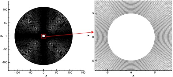
Gridgen was used to generate grids, as shown in Fig. 2. Two-dimensional grids were adopted. 401 grid points were arranged in the radial direction. 361 grid points were arranged in the circumferential direction. Radial grids around the cylinder surface were locally encrypted and gradually enlarged according to the scale factor of 1.05 times. Finally, there were 350954 elements and 387903 nodes in this model. The material is steel of the studied cylindrical model, so the Elastic Modulus is 2.1e11 Pa, the Poisson’s ratio is 0.3, and the density is 7800 kg/m3. The medium is air, so the sound velocity is 340 m/s.
Fig. 2Schematic diagram for the grids of a circular cylinder
4.1.2. Analysis on numerically computational results
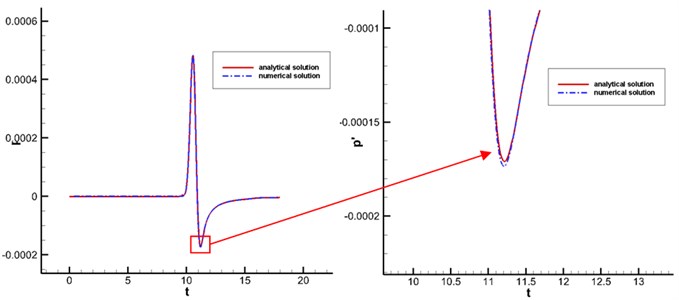
Fig. 3 displayed contours for the pressure fluctuation obtained by numerical and analytical computation. Fig. 4 showed the pressure fluctuation with time at observation points obtained by analytical and numerical computation. As displayed from Fig. 4, the maximum and minimum pressure values of analytical results were 0.0005 Pa and –0.0005 Pa respectively. The maximum and minimum values of numerical computational results were 0.00049 Pa and –0.00049 Pa. It indicated that two kinds of methods presented a good agreement, which verified the correctness of numerical simulation method in this paper.
Fig. 3Computational results of contours for pressure fluctuation at a certain moment
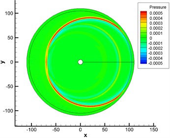
a) Analytically computational results
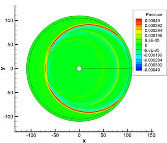
b) Numerically computational results
Fig. 4Change of pressure fluctuations with time at observation points
4.2. Propagation computation of monopole sound source in shear flow
4.2.1. Sound source model and grid generation of acoustic computation
To observe the propagation of sound wave in the shear layer more clearly, this paper adopted monopole as sound source and computed its propagation process in the shear layer. Below was the model for monopole sound source used in this paper. was sound source term at the right end of LEE in Eq. (3):
wherein, , referred to the magnitude and frequency of pressure fluctuation; was the half width of Gaussian function; was an adjustable parameter.
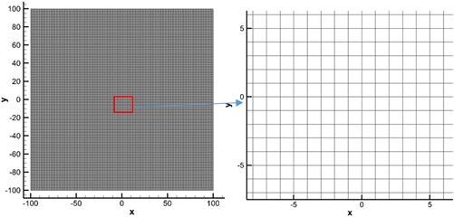
Gridgen was used to generate grids, as shown in Fig. 5. Two-dimensional structured grids were applied. Computational domain was and . 200 grid points were arranged in the and directions. Uniform grids were adopted. Grid spacing was 1 m.
Fig. 5Schematic diagram for the computational grids of monopole sound source propagation
4.2.2. Analysis of numerical computational results
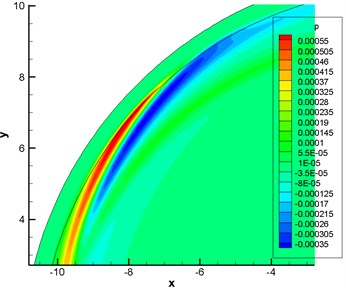
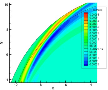
Fig. 6 displayed the contour for the distribution of Mach number under the background of a shear layer. Fig. 7 showed the contour for pressure fluctuation of monopole sound source obtained by the numerical simulation of LEE in the static atmospheric layer and shear layer. Through comparison, it could be seen that sound wave had refraction effect around the shear layer. Therefore, acoustic perturbation after refraction and acoustic perturbation produced by sound source formed very obvious interference fringes around the shear layer.
The shear layer had an impact on the propagation path of sound and the amplitude and frequency of sound pressure in the process of sound propagation. When sound wave was transmitted through the shear layer, it would cause refraction loss. In the meanwhile, sound ray diffused after going through the shear layer under the action of refraction. To keep energy conservation, sound energy was reduced in the unit area, which resulted in changes in the amplitude of sound pressure in the sound field.
Fig. 6Contour for the Mach number of flow field in the shear layer
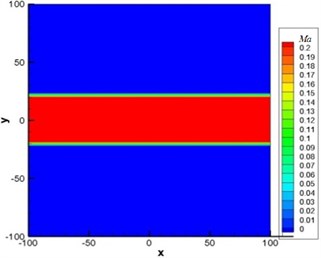
a) Without the shear layer
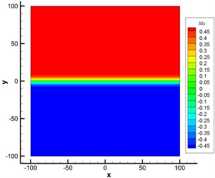
b) With the shear layer
Fig. 7Numerical computation for the sound propagation of monopole sound source
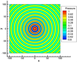
a) Without the shear layer
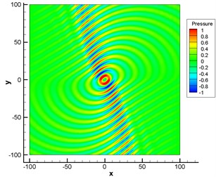
b) With the shear layer
4.3. Computation of different modes of sound sources of engine duct in the shear layer
4.3.1. Sound source model and grid generation of acoustic computation
Engine tailpipe nozzle could be considered as a cylindrical pipe. Therefore, the computational method for the sound source of cylindrical pipe could be adopted to conduct numerical computation for the single mode and multi-mode sound propagation of engine tailpipe nozzle. The specific derivation of sound source under the mode of cylindrical pipe adopted in this paper was as follows:
From the sound theory of pipe, it could be seen that corresponding (, ) secondary wave could be stimulated in the pipe when the excitation frequency of sound source was higher than some normal frequency . Therefore, the first minimum normal frequency except for zero was called as the cut-off frequency of sound wave pipe, the cut-off frequency of pipe for short. If the frequency of sound source was lower than that of pipe, the only (0, 0) secondary wave could be transmitted in this pipe.
In the computation of sound propagation, sound source should be known. Therefore, sound source in the pipe should be expressed firstly before the computation of sound propagation. It was mainly a cylindrical pipe. In addition, suppose pipe wall was rigid, wave equation in three-dimensional rectangular coordinate was:
Below was the relationship between rectangular and cylindrical coordinates:
Laplace operator of the cylindrical coordinate could be expressed as:
Therefore, wave equation could be transformed into the following form:
. Wherein, was function about ; referred to function about ; stood for function about ; represented sound velocity. After they were substituted into the transformed wave equation, three ordinary differential equations could be obtained as follows:
wherein, referred to wave number in the radial direction; stood for wave number in the circumferential direction; . For equation, traveling wave solution was obtained:
As the relationship of should be satisfied, in the equation had to be a positive integer. For equation, . The equation was transformed into:
It was a standard Bessel equation of m order, whose general solution could be expressed as the following form:
wherein, , was Bessel function; two coefficients including and could be solved by boundary and initial conditions. Finally, the non-dimensional sound pressure of pipe sound source could be expressed as follows:
wherein, referred to wave number in the radial direction. From the basic nature of sound wave, the pulsating quantity of velocity in the Cartesian coordinate system could be expressed as:
, , was used to represent the axial, radial and circumferential pulsating quantities of velocity of sound wave in the circular pipe. Then:
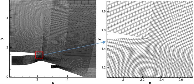
Gridgen was used to generate grids, as shown in Fig. 8. Structured grids of two-dimensional multi-block joint were adopted. As sound source was defined in the duct, grids in the duct were locally encrypted. In addition, grids at the exit of duct were also encrypted locally due to the refraction effect of the shear layer at the exit of duct. As shown in Fig. 8, quadrilateral elements were adopted to divide this model. Finally, there were 890923 elements and 930891 nodes in the computational model.
Fig. 8The computational grids of sound source propagation of engines
4.3.2. Analysis on numerically computational results
Mach number was 0.3 at the nozzle. Numerical simulation was conducted for the flow field through solving RANS equation to obtain the contour for the distribution of Mach number under the background of the shear layer, as shown in Fig. 9(b). It could be seen from the figure that there was a strong shear layer at the exit of duct.
Fig. 9Contour for Mach number under the background of engine wake flow
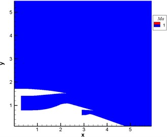
a) Without the shear layer
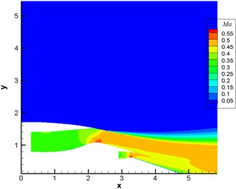
b) With the shear layer
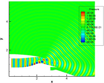
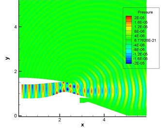
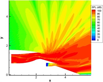
Fig. 10 displayed the computational result of pressure fluctuation of sound source in the single pipe mode 0, 0 (namely plane wave). Fig. 11 displayed the computational result of pressure fluctuation of sound source in the single pipe mode 4, 1. Fig. 12 displayed the computational result of pressure fluctuation of sound source in the multi-pipe mode 4, 1-4. referred to circumferential mode while n stood for radial mode. As displayed from Fig. 10 to Fig. 12, the propagation of sound inside the duct was regular to some degree in the single mode and a little disorderly in the multi-mode situation. Without the shear layer, sound wave was mainly transmitted along the flow direction at the exit of duct. When there was a strong shear layer in the flow field, the energy amplitude and especially propagation direction of sound wave would see some changes at the exit of duct. For plane wave, the refraction effect of the shear layer was the most obvious. The existence of the shear layer led to the upper and lower deviation of sound wave transmitted to the right side. In addition, pressure contour lines were uniformly spaced vertical lines within the range of for plane wave and the single pipe mode. As the inner wall of air inlet was approximately horizontal here, sound wave seemed to be transmitted in the circular pipe without shear flow. After entering the air inlet, sound wave was mainly transmitted along the positive direction of axis. Inside the air inlet and in the area of open boundary near the left side, intervals between wave peaks were very uniform and exactly equal to non-dimensional wavelengths.
Fig. 10Computational result of pressure fluctuations of engine duct (pipe mode m= 0, n= 0)
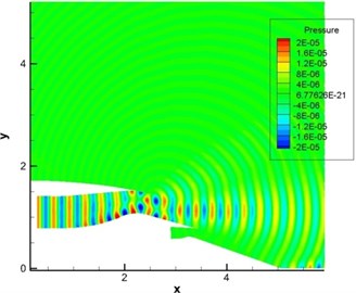
a) Without the shear layer
b) With the shear layer
Fig. 11Computational result of pressure fluctuations of engine duct (pipe mode m= 4, n= 1)
a) Without the shear layer
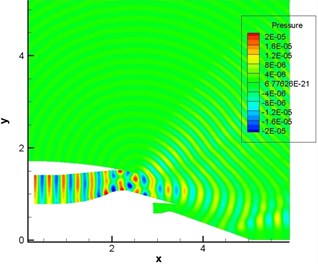
b) With the shear layer
Fig. 12Computational result of pressure fluctuations of engine duct (pipe mode m= 4, n= 1-4)
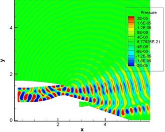
a) Without the shear layer
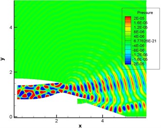
b) With the shear layer
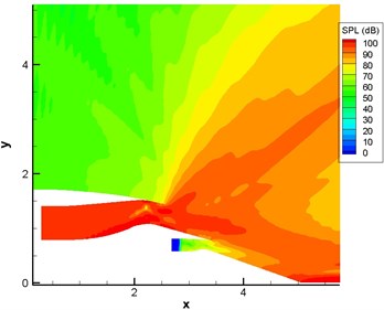
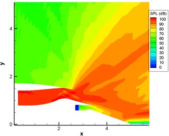
Fig. 13 displayed the computational result of sound pressure level of sound source in the single pipe mode 0, 0 (namely plane wave). Fig. 14 displayed the computational result of sound pressure level of sound source in the single pipe mode 4, 1. Fig. 15 displayed the computational result of sound pressure level of sound source in the multi-pipe mode 4, 1-4. As displayed from Fig. 12 to Fig. 15, sound pressure levels were uniform inside the duct and showed slight changes only in the multi-pipe mode. Outside the duct, sound pressure levels were obviously and unevenly distributed. For the single pipe mode, the direction of sound radiation was rather centralized; for the multi-pipe mode, the radiation of sound radiation was rather dispersive. In addition, the dispersive-ness of sound radiation became stronger and stronger with the increasing number of pipe modes. In addition to this, it could also be found that the shear layer at the exit of duct mainly led to the upward deviation of sound radiation. For plane wave, the deviation effect was particularly obvious. In addition, the existence of the shear layer reduced the dispersion characteristics of sound source in the pipe mode in the direction of sound radiation outside the pipe because the viscosity of the shear layer could attenuate energy in the process of sound propagation.
Fig. 13Computational result of sound pressure levels of engine duct (pipe mode m= 0, n= 0)
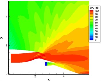
a) Without the shear layer
b) With the shear layer
Fig. 14Computational result of sound pressure levels of engine duct (pipe mode m= 4, n= 1)

a) Without the shear layer
b) With the shear layer
Fig. 15Computational result of sound pressure levels of engine duct (pipe mode m= 4, n= 1-4)
a) Without the shear layer
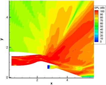
b) With the shear layer
Fig. 16 displayed the directivity patterns of sound with and without the shear layer in different pipe modes. It was clear that the radiation direction of sound wave was mainly between 0° and 30° without the shear layer and between 50° and 80° with the shear layer for single pipe mode 0, 0 (namely plane wave). For the single pipe mode 4, 1, the change rule in the direction of sound radiation was similar to that of plane wave. However, sound pressure level sharply increased from 0 to 92 dB between 0° and 10°. For the multi-pipe mode 4, 1-4, the radiation direction of sound wave was mainly between 20° and 40° and had obvious dispersion effect between 60° and 120° without the shear layer. Namely, sound directivity was distributed like a petal. Fig. 15(a) also showed that the contour for sound pressure level had many obvious dispersion effects between 60° and 120°. When there was a shear layer, the radiation direction of sound wave was mainly around 60°. In addition, there was no obvious dispersion effect between 60° and 120°. Fig. 15(b) also showed obvious sound directivity in the direction of 60° and weak sound directivity at other angles.
Fig. 16Sound directivities of sound source modes of different pipes with and without the shear layer
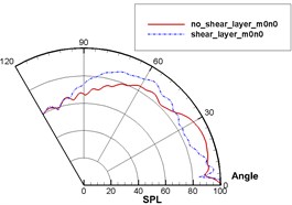
a) 0, 0
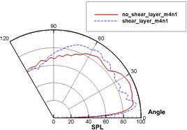
b) 4, 1
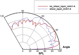
c) 4, 1-4
5. Conclusions
This paper verified the correctness of numerical simulation method through solving linearized Euler equations and verification example. Based on the verified model, this paper analyzed the propagation mechanism of aerodynamic noises in the shear layer through computing the propagation of monopole sound source and the propagation of different modes of sound sources of engine duct, studied the impact of shear flow on sound propagation and obtained the following conclusions:
1) The treatment for aero-acoustics with space-time and high-precision dispersion scheme, nonreflecting boundary condition and numerical filtering in this paper could satisfy the requirements of computational aero-acoustics and obtain reasonable numerically computational results.
2) The shear layer had an impact on the propagation path of sound and the amplitude of sound pressure in the process of sound propagation. When sound wave was transmitted in the shear layer, it would cause refraction loss. In the meanwhile, sound ray diffused after going through the shear layer under the action of refraction. To keep energy conservation, sound energy was reduced in the unit area, which thus resulted in changes in the amplitude of sound pressure in the sound field.
3) For different modes of pipe sound sources, the shear layer would produce different refraction effects. For plane wave, the refraction effect produced by the shear layer was the most obvious.
4) For the single pipe mode, the radiation of sound radiation was rather centralized; for the multi-pipe mode, the radiation of sound radiation was rather dispersive. In addition, the dispersive-ness of sound radiation became stronger and stronger with the increasing number of pipe modes. Namely, the directivity pattern of sound seemed to be a petal. The existence of the shear layer would reduce the dispersion effect of multi-pipe modes in the direction of sound radiation.
5) Sound propagation was affected by non-uniform flow to a large extent. When the noise problem caused by turbulent flow was numerically studied, therefore, the impact of such non-uniform shear flow should be taken seriously so as to obtain correct results.
References
-
Wang Z., Vong S. Compact difference schemes for the modified anomalous fractional sub-diffusion equation and the fractional diffusion-wave equation. Journal of Computational Physics, Vol. 277, 2014, p. 1-15.
-
Liu J. L., Zhang J. Y., Zhang W. H. Study of computational method of far-field aerodynamic noise of a high-speed train considering ground effect. Chinese Journal of Computational Mechanics, Vol. 30, Issue 1, 2013, p. 94-100.
-
Bispen G., Lukáčová Medvid’ová M., Yelash L. Asymptotic preserving IMEX finite volume schemes for low Mach number Euler equations with gravitation. Journal of Computational Physics, Vol. 335, 2017, p. 222-248.
-
Garipova L. I., Garipova L. I., Batrakov A. S., et al. Aerodynamic and acoustic analysis of helicopter main rotor blade tips in hover. International Journal of Numerical Methods for Heat and Fluid Flow, Vol. 26, Issue 7, 2016, p. 2101-2118.
-
Trask N., Maxey M., Hu X. Compact moving least squares: An optimization framework for generating high-order compact meshless discretizations. Journal of Computational Physics, Vol. 326, 2016, p. 596-611.
-
Morgan B. E., Greenough J. A. Large-eddy and unsteady RANS simulations of a shock-accelerated heavy gas cylinder. Shock Waves, Vol. 26, Issue 4, 2016, p. 355-383.
-
Groves K. H., Lennox B. Directional wave separation in tubular acoustic systems – the development and evaluation of two industrially applicable techniques. Applied Acoustics, Vol. 116, 2017, p. 249-259.
-
Joshi S. M., Chatterjee A. Higher-order multilevel framework for ADER scheme in computational aeroacoustics. Journal of Computational Physics, Vol. 338, 2017, p. 388-404.
-
González A. S., Aparicio J. R. F. Turbine tone noise prediction using a linearized computational fluid dynamics solver: comparison with measurements. Journal of Turbomachinery, Vol. 138, Issue 6, 2016, p. 061006.
-
Sassanis V., Sescu A., Collins E. M., et al. A hybrid approach for nonlinear computational aeroacoustics predictions. International Journal of Computational Fluid Dynamics, 2017, p. 1-20.
-
Rona A., Spisso I., Hall E., et al. Optimized prefactored compact schemes for linear wave propagation phenomena. Journal of Computational Physics, Vol. 328, 2017, p. 66-85.
-
Mao M., Jiang Y., Deng X., et al. Noise prediction in subsonic flow using seventh-order dissipative compact scheme on curvilinear mesh. Advances in Applied Mathematics and Mechanics, Vol. 8, Issue 2, 2016, p. 236-256.
-
Masovic D., Zotter F., Nijman E., et al. Directivity Measurements of Low Frequency Sound Field Radiated from an Open Cylindrical Pipe with a Hot Mean Flow. SAE Technical Paper, 2016.
-
Hamiche K., Gabard G., Bériot H. A high-order finite element method for the linearised Euler equations. Acta Acustica united with Acustica, Vol. 102, Issue 5, 2016, p. 813-823.
-
Snakowska A., Jurkiewicz J., Gorazd Ł. A hybrid method for determination of the acoustic impedance of an unflanged cylindrical duct for multimode wave. Journal of Sound and Vibration, Vol. 396, 2017, p. 325-339.
-
Çınar Ö. Y., Boij S., Çınar G., et al. Sudden area expansion in ducts with flow – A comparison between cylindrical and rectangular modelling. Journal of Sound and Vibration, Vol. 396, 2017, p. 307-324.
-
Livebardon T., Moreau S., Gicquel L., et al. Combining LES of combustion chamber and an actuator disk theory to predict combustion noise in a helicopter engine. Combustion and Flame, Vol. 165, 2016, p. 272-287.
-
Zhang N., Hua X. I. E., Xing W., et al. Computation of vertical flow and flow induced noise by large eddy simulation with FW-H acoustic analogy and Powell vortex sound theory. Journal of Hydrodynamics, Series B, Vol. 28, Issue 2, 2016, p. 255-266.
-
Zhu Z., Zhao Q. Optimization for rotor blade-tip planform with low high-speed impulsive noise characteristics in forward flight. Proceedings of the Institution of Mechanical Engineers, Part G: Journal of Aerospace Engineering, 2016, https://doi.org/10.1177/0954410016650908.
-
Jain R. K., Yeo H., Ho J. C., et al. An assessment of RCAS performance prediction for conventional and advanced rotor configurations. Journal of the American Helicopter Society, Vol. 61, Issue 4, 2016, p. 1-12.
-
Ho J. C., Yeo H., Bhagwat M. Validation of rotorcraft comprehensive analysis performance predictions for coaxial rotors in hover. Journal of the American Helicopter Society, Vol. 62, Issue 2, 2017, p. 1-13.
-
Zhang J., Chu W., Zhang H., et al. Numerical and experimental investigations of the unsteady aerodynamics and aero-acoustics characteristics of a backward curved blade centrifugal fan. Applied Acoustics, Vol. 110, 2016, p. 256-267.
-
Mohamed M. H. Reduction of the generated aero-acoustics noise of a vertical axis wind turbine using CFD (computational fluid dynamics) techniques. Energy, Vol. 96, 2016, p. 531-544.
-
Balduzzi F., Drofelnik J., Bianchini A., et al. Darrieus wind turbine blade unsteady aerodynamics: a three-dimensional Navier-Stokes CFD assessment. Energy, 2017.
-
Octavianty R., Asai M. Effects of short splitter plates on vortex shedding and sound generation in flow past two side-by-side square cylinders. Experiments in Fluids, Vol. 57, Issue 9, 2016, https://doi.org/10.1007/s00348-016-2227-4.
-
Oguma Y., Fujisawa N. Sound source measurement of a semi-circular cylinder in a uniform flow by particle image velocimetry. Journal of Flow Control, Measurement and Visualization, Vol. 4, Issue 4, 2016, p. 162-170.
-
Zheng H., Wang J. Numerical study of galloping oscillation of a two-dimensional circular cylinder attached with fixed fairing device. Ocean Engineering, Vol. 130, 2017, p. 274-283.
-
Komatsu R., Iwakami W., Hattori Y. Direct numerical simulation of aeroacoustic sound by volume penalization method. Computers and Fluids, Vol. 130, 2016, p. 24-36.
-
Wall A. T., Gee K. L., Neilsen T. B., et al. Military jet noise source imaging using multisource statistically optimized near-field acoustical holography. The Journal of the Acoustical Society of America, Vol. 139, Issue 4, 2016, p. 1938-1950.
-
Ning F., Wei J., Qiu L., et al. Three-dimensional acoustic imaging with planar microphone arrays and compressive sensing. Journal of Sound and Vibration, Vol. 380, 2016, p. 112-128.
-
Mo P., Jiang W. A hybrid deconvolution approach to separate static and moving single-tone acoustic sources by phased microphone array measurements. Mechanical Systems and Signal Processing, Vol. 84, 2017, p. 399-413.
About this article

This study is partially supported by Natural Science Foundation of Hunan Province (No. 2016JJ4012) and by the Key Built Disciplines of Hunan University of Finance and Economics.
