Loss factor estimation of the plywood materials

1. Introduction

There are several methods to analyze structural damping behavior of the materials. One of the damping loss factors (DLF) identification method is Oberst Beam Method [1], where specimen is fixed on one side and other side is excited. The excitation is introduced by an electro-magnetic induction at free end. Damping estimation is then related to identification of the frequency bandwidth using half-power (–3 dB) points around the resonances of transmissibility spectrum. The disadvantage of this method might be in excitation of non-metallic materials and damping estimation for closely spaced (higher order) modes, where modal overlap will affect frequency bandwidth identification. Oberst Beam Method is not applicable for so called in-situ panels damping estimation, where damping mechanism is influenced by attached structures, shape, profile, variable sections etc.

Another DLF identification method, Power Injection Method (PIM) [5], use stationary broad-band force excitation and set of accelerometers randomly placed on the panel. This method defines the DLF as the ratio between dissipated energy and total energy per radians of motion. This method requires the stabile stationary force exciter.

The effective method, based on time domain frequency response of the impact force pulse, is called Decay Rate Method (DRM) [4]. This method is based on the force impulse performed by the impact hammer and response at mounted accelerometers array, randomly installed on the panel(s) or whole structural body. The main advantage of this method is the identification of the in-situ damping as close as possible to real scenario and practically with no limit on specimen dimensions. The complexity of identified objects is not a hindrance for the damping behavior estimation. The potential problems in practical application might arise from proper accelerometers sensitivity selection and force sensor inside the impact hammer to get the relevant magnitude spectrum with the appropriate signal to noise distance. The recommended accelerometer sensors are low weight, which do not affect panel behavior, but their very small weight of the seismic mass causes the signal distortion in the low band measurement. The recommended impact hammer uses the charge force sensor, because of the increased sensitivity for shock pulses. The impact hammer impulses show the stochastic behavior. There is necessary to perform sufficient number of measurements, to get reasonable ensemble average important for statistical relevance. Since damping loss factor estimation is related to response of resonant modes, theoretically all modes should be excited to get correct panel damping. For this reasons it is necessary to perform couple of random accelerometers locations and random impacts on each panel.

The comparison between the PIM and DRM describes [2, 3] and presents good results when there are modes within the analyzed frequency band. The both methods give similar results. PIM showed to be less accurate at low frequencies bandwidth. The PIM has a strong dependency on the amount of the response points. The DRM method uses the initial decay of the impulse response and can be faster than PIM because it estimates little quantities of FRF. The usage of DRM seems to be limited to lightly damped structures, for DLF < 0.1 (where 1 = 100 %). The limitation is related with frequency bandwidth filter used when filtering FRF to estimate time decay for particular Third Octave Frequency point.

The DRM method was used for the DLF estimation of the plywood panels. This article shows the loss factor identification for one plywood panel with the statistical dispersion of results. The influence on the dispersion value has several causes.

2. Measurement

The specified trigger activates the start of the measurement and is set on the level 50 N of the loading edge of the impact hammer force. The beginning of the measurement is set to 2 ms before the trigger activation time to avoid the loss of the information about the loading edge of the impact hammer force. Six acceleration sensors were randomly distributed and glued to the specimens by the silicone wax.

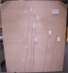
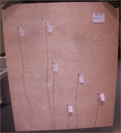
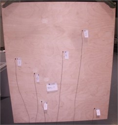
Hammer impact (tap) was performed always as close as possible to every acceleration sensor. Force and accelerations signals were recorded per each individual hammer impact. Measurement has been repeated three times per each plywood panel, where acceleration sensor has been re-position between each measurement set, to ensure highest signal decay variety (Fig. 1).

Plywood panel was hanged on the soft suspension to ensure the free-free modes.

Fig. 1Plywood panel with different accelerometer distributions

3. Estimation

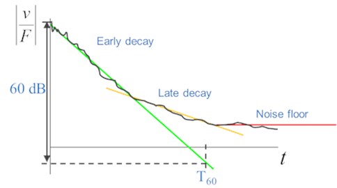
DRM methodology, also called T60 Reverberation time, has been used for 1/3 Octave damping loss factor (DLF) estimation. The principle of this approach is to identify T60 time decay needed for an impact response to drop by 60 dB compared to initial peak value. Time decay is evaluated per each frequency band separately. Thereafter the damping is then defined as relation:

The damping $\eta$ corresponds to the damping at 1/3 Octave Central Frequency $f$ and estimated decay time $T_{60}$. Then 1/3 Octave filter is applied on each time signal per each frequency separately:

From the filtered time signal an energy envelope is created and after that the curve slope is determined:

Evaluation is made at each sensor position independently. Positions of the sensors are chosen randomly in such way, that the maximum number of structural modes could be excited. Then hammer impact is applied at each sensor position. This will populate 6 (6 accelerometers) response signals per one impact position, repeating this for six impact positions will result in 36 DLF curves per single measurement. By averaging evaluated DLF’s curves, a final DLF curve is obtained:

where $M$ is the number of all the positions and $N$ is number of impacts.

Fig. 2DRM estimation

During the measurement six acceleration sensors were available. Each set of measurements consists of six measurements for one configuration. Final results are both the average of damping value in the 1/3 Octave band and its linearized damping representation which will be used in future simulations.

DRM methodology is shown as the step by step description:

1. Antialiasing filtering of the force and acceleration signals;

2. Force and acceleration spectrum by using FFT;

Fig. 3Force magnitude spectrum

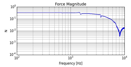
3. FRF estimation from the Force and the relevant acceleration spectrum in complex form;

4. Inverse FFT estimation – transformation of FRF from frequency to time domain;

5. Signal filtering across the 1/3 Octave band;

6. Envelope estimation of the early decay; Identification of the $T_{60}$ in 60 dB decrease.

Fig. 4FRF function as spectrum

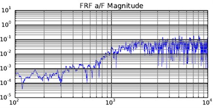
Fig. 5FRF function in time domain form

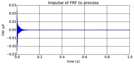
Fig. 6Decay rate in 100 Hz and 1000 Hz

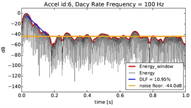
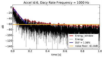
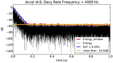
Fig. 7Decay rate in 4000 Hz and DLF estimation across the 1/3 octave band

4. Statistics

The statistics analysis is suitable cause of relevant output for the sensors array estimations. The loss factor dispersion is helpful information for the sensitivity analysis of the damping behavior. The loss factor dispersion of the plywood panels influence panel vibrations and panel radiation representation in numerical models, what consequently cause dispersion of the acoustic results. It is mandatory to use some stochastic method for the virtual simulation like the loss factor generation from the relevant distribution in consistent finite element models.

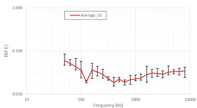
Fig. 8DLF estimation across the 1/3 Octave band for different sensor distributions

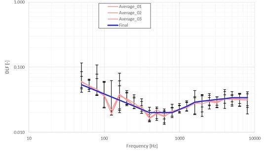
The equal input conditions are necessary for the statistics analysis. The loss factor estimation sensitivity depends on the sensor distribution. The loss factor estimation is performed for each of 6 hammer impact for 5 accelerometer sensors. The statistic sample contains 30 values of the loss factor.

The statistical analysis is suitable to perform across the 1/3 Octave band for each sensor distribution. The output of the analysis is histogram of the estimated loss factor with the possible substitution of the appropriate distribution.

The loss factor distribution for the lower frequency modes (lower than 200 Hz) evinces the larger values. The loss factor histograms for 100 Hz and 1000 Hz are shown on Fig. 9.

Fig. 9DLF histogram for 100 Hz and 1000 Hz

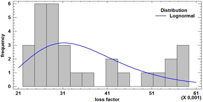
a) 100 Hz

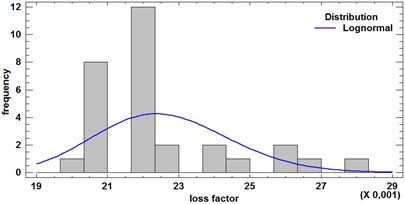
b) 1000 Hz

The results show that the lognormal is more suitable than the normal distribution for the substitution.

The appropriate theoretical distribution for experimental data has been found using Kolmogorov-Smirnov (also K-S) goodness of fit test. It tests null hypothesis $H_0$ saying that the selection $X_1$,…, $X_n$ comes from distribution $\mathrm{\Phi }\left(x\right)$. The statistics is calculated from Eq. (6), where $F_n\left(x\right)$ is selective distribution:

In case $D_n\ge D_n\left(\alpha \right)$, where $D_n\left(\alpha \right)$ is tabulated critical value, we can reject $H_0$ with level of significance $\alpha$. In comparison with Pearson ${\chi }^2$ goodness of fit test, the advantage of K-S test lies in possibility of usage also in case of small sample of data and in case of empty classes of histogram.

The K-S tests shown that the experimental values of loss factor come from lognormal distribution which is given by Eq. (7):

where $\mu$ is mean and $\sigma$ is standard deviation, which represent parameters of the lognormal distribution $LN\left(\mu ,\sigma \right)$. The tests have been done using statistical software Statgraphics Centurion XVI.

5. Conclusions

The loss factor estimation of the plywood material is possible to get by using the Decay Rate Method. This method enables the easy identification of the plywood panel behavior with the impact hammer response close to the real conditions. The relevant virtual analysis enables the stochastic designation of the DLF with the lognormal distribution. The relevant stochastic dispersion seems to be effective for the sensitivity analysis of the complex model on the separate part as the plywood panel behavior in term of the acoustic reduction analysis in virtual environment. The dispersion of the DLF causes the sensitivity of used sensors like the distortion in the low band or the small signal to noise distance in high band frequencies and inhomogeneity of the plywood panel like the structural behavior dispersion.

References

-
Petřík J., Pašek M., Šašek J., Kulhavý P. Vibration and noise reduction analysis of sheet metal structures with damping layer. Applied Mechanics and Materials, Vol. 732, 2015, p. 291-296.
Bratti G., Montenegro M. A. G., Lenzi A., Jordan R., Cordioli J. A. Estimation of damping loss factor of fuselage panel by power injection method and impulse response decay method. Proceeding of COBEM, 2011.
Cabell R., Schiller N., Allen A., Moeller M. Loss factor estimation using the impulse response decay method on a stiffened structure. INTER-NOISE, 2009
Ewing M. S., Dande H., Vatti K. Validation of panel damping loss factor estimation algorithms using a computational model. 50th AIAA/ASME/ASCE/AHS/ASC Structures, Structural Dynamics, and Materials Conference, 2009.
Maxit L., Guyader J. L. Estimation of SEA coupling loss factors using a dual formulation and FEM modal information. Journal of Sound and Vibration, 2001, p. 907-930.
About this article
This publication was written at the Technical University of Liberec as part of the Project “Innovation of Products and Equipment in Engineering Practice” with the support of the Specific University Research Grant, as provided by the Ministry of Education, Youth and Sports of the Czech Republic in the year 2016.