Abstract
A modified stochastic averaging method on a Duffing-Rayleigh oscillator with strongly nonlinearity subject to Gaussian colored noise excitation was proposed. The so-called He’s energy balance method was applied to obtain the averaged frequency of the conservative system. Subsequently, the stochastic averaging method of strong nonlinearity was used. The modified method can offer more concise approximate expressions of the drift and diffusion coefficients without weakening the accuracy of predicting the responses of the systems too much. The stationary responses of probability density of amplitudes, together with joint probability density of displacement and velocity are studied to verify the presented approach. The reliability of the systems was also investigated to offer further support. Digital simulations were carried out and the output of that are coincide with the theoretical approximations well.
1. Introduction
In recent half century, stochastic vibration has drawn accelerating interests. An effective and powerful method dealing with stochastic vibrations is the stochastic averaging method. The stochastic averaging method initialized by Landau and Stratonovich [1] and Khasminskii [2] is also called as the method of quasi-conservative averaging. Later, Zhu and Lin [3, 4] re-derived an approach named the stochastic averaging of energy envelope by taking into account of the conservative part of the Wong-Zakai correction terms of the system. This prevalent approach has been used and developed by many researchers [5-12]. The responses of the single-degree-of freedom (SDOF) or multi-degree-of-freedom (MDOF) systems subject to non-white wide-band random excitation [6-8] or combined harmonic and white noise [10] have all been studied in detail. After that, Zhu [11, 12] extended the stochastic averaging of energy envelope method into Hamilton systems.
Xu and Chung [13] have proposed a method to deal with noise-free strongly nonlinear Oscillators based on the so-called generalized harmonic functions. This method has been extended by Zhu and Huang [14, 15] to handle strongly non-linear oscillators with lightly linear and (or) non-linear damping subject to weakly external and (or) parametric excitations of wide-band random processes. The key technique of the Zhu and Huang’s method is using expressions of the displacement and velocity as: , , where is the instantaneous frequency and is the amplitude. The frequency can be averaged to by expending it into a string of Fourier series and integrating them with respect to form 0 to . A typical Duffing-Vanderpol oscillator has been studied by this method [15], the stability of the stationary response and the stochastic Hopf-bifurcation has been investigated. The precision of this method has been verified by digital simulations. However, this method is less than flawless in view of the fact that it yields very long expressions of drift coefficient and diffusion coefficient which are quite time consuming during calculations. Thus, there remains a need to shorten the expressions of the drift coefficient and diffusion coefficient without weakening the accuracy too much. Furthermore, this method is mainly applied on white noise or non-white wide-band random excitations, we try to extend this method to oscillators under colored noise excitations.
In this paper, a Duffing-Rayleigh oscillator under colored noise excitation was studied as a representative example. A so-called energy balance method calculating the averaged frequency of conservative systems proposed by He [16] has been used to obtain concise expression of the averaged . The feature of the method is constructing the Hamilton of the system and keeping the input and the output of it in balance. This method has been extended by many researches into non-conservative systems [17-21] and the accuracy has been proved to be good enough. In the following sections, The Zhu and Huang’s method was modified by the He’s energy balance method. The stationary probability density function (PDF) of amplitude and the joint probability of the displacement and velocity were given simultaneously based on the shortened frequency . The reliability and the first passage failure were also studied to offer further support. Digital simulations were carried out and the results were consistent with the theoretical approximations.
2. Stochastic averaging method
A Duffing-Rayleigh oscillator with light damping and colored noise excitation was presented as follows. The linear and nonlinear damping coefficients are assumed to be of order, , , the excitation is assumed to be of order:
As well known, the colored noise can be obtained by a white noise passing through a linear filter:
where denotes the correlation time and denotes a Gaussian white noise with 0 mean and intensity of 2. The correlation function of is:
The conservative system of Eq. (1) is:
The Hamilton and the potential energy are given as:
where is the total energy of the oscillator while is the potential energy.
Assuming all the trajectories in domain of phase plan () are periodic surrounding (0, 0). The approximate periodic solution of Eq. (1) can be written as:
where:
in which is the amplitude of displacement, which is related to as follows:
and is the instantaneous frequency of the oscillation. For the convenience of calculating, the instantaneous frequency can be transformed to be the averaged frequency by the He’s energy balance method [16].
For , we get , , substituting it into Eq. (7) yields the Hamilton . Then, replacing by in Eq. (8) and substituting it into Eq. (7) yields the Hamilton . we obtain the following residual equation:
Since Eq. (7) is only an approximation to the exact solution, cannot be made zero everywhere. Collocation at , we get:
By letting equals to zero, we can get the averaged frequency :
For Eq. (1) we can use the following approximate relation:
where is the phase.
With the transformations accomplished, Eq. (1) becomes:
where:
Eq. (14) is of standard form. converges weakly to a diffusive Markov process even in a semi-infinite time interval. The Ito equation of the limiting diffusion process is of the form:
where the drift coefficient and the diffusion coefficient are as follows:
is the standard unit Brown's motion, is averaging with respect to time, is the correlation function. For white noise, it is well known that:
we can obtain the following drift and diffusion coefficients of stochastic equations for amplitude :
3. Stationary probability density function
The averaged Fokker-Plank-Kolmogorov (FPK) equation associated with Ito Eq. (15) is of the form:
where is the transition probability density of displacement amplitude nontrivial stationary solution exists due to non-vanishing of external excitation. Under assumption of zero probability flow at the two boundaries and , the stationary solution of FPK Eq. (19) for system Eq. (15) is of the form:
where constant is the normalization constant.
Substituting Eq. (18) into Eq. (20) yields:
The stationary probability density of total energy or energy envelope can be obtained as follows:
where:
is the inverse function of .
The stationary probability density of displacement and velocity can be further obtained from as follows:
where can be obtained from by the transformation .
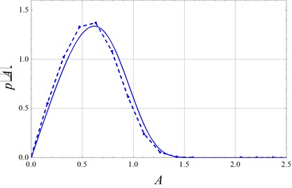
Fig. 1Stationary probability density function of amplitude A (solid lines: stochastic averaging Eq. (21); Dashed lines: method in reference [15]; dots: digital simulation)
![Stationary probability density function of amplitude A (solid lines: stochastic averaging Eq. (21); Dashed lines: method in reference [15]; dots: digital simulation)](https://static-01.extrica.com/articles/17011/17011-img1.jpg)
a)
![Stationary probability density function of amplitude A (solid lines: stochastic averaging Eq. (21); Dashed lines: method in reference [15]; dots: digital simulation)](https://static-01.extrica.com/articles/17011/17011-img2.jpg)
b)
Comparisons of theoretical analysis and digital simulation were displayed in Fig. 1 and Fig. 2. The damping coefficients were set as 0.1, 0.1, the nature frequency was set as 1, and the nonlinear stiffness coefficient was set as . The densities of white noise were set as 0.5 and 1.0, and the correlation time was set as and 10, respectively. Totally 1 000 sets of white noise were imposed to the system Eq. (1). Each set noise includes 20 000 numbers. The numerical solutions of the oscillator Eq. (1) could be obtained by an order-2 stochastic Runge-Kutta algorithm [22]. The last 10 000 dots were kept as the steady state responses. The stationary probability density function (PDF) of the amplitude with different and same was shown in Fig. 1(a). As we know, large noise density leads to large horizontal coordinate of the peak of PDF and low peak value . Also, the stationary probability density function of the amplitude with different and same was illustrated in Fig. 1(b). The solid lines were results obtained by the proposed method in this paper and the dashed lines were given by the method in reference [15]. We have to admit that the method in reference [15] offered better accuracy than the method we used in this paper. But, it was also obvious that the presented method can offer acceptable analytical approximate solutions in view of the fact the solid lines were quite against the dashed lines except for the peak positions. Furthermore, considering the reduction of the calculation and the error between the dashed line and the digital results was negligible, the presented method is valid and effective. It is obvious that larger time delay coefficient results in wider diffusion range of amplitude.
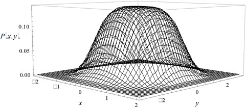
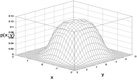
The joint probability of the displacement and velocity is shown is Fig. 2, where Fig. 2(a) is the theoretical result given by Eq. (23) and the Fig. 2(b) is the digital simulation result, with parameters set as 0.5 and . It is seen that the analytical results are fairly in agreement with those from digital simulation.
Fig. 2The joint probability of the displacement and velocity: a) theoretical result, b) digital simulation result
a)
b)
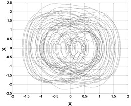
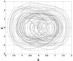
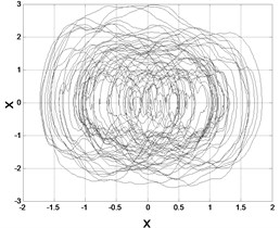
To give a intuitive impression of the system excited by colored noise, three samples of the phase trajectory were illustrated in the Fig. 3. It is obvious that both the large noise density and large correlation time lead to thickly cycles of trajectory spreading wider. This phenomenon can be seen clearly in Fig. 1. The peaks of the stationary probability density functions were drifted to the right side of the coordinate with noise density and large correlation time increased.
Fig. 3Samples of Phase trajectories: a) D= 0.5, λ= 2, b) D= 1, λ= 2, c) D= 0.5, λ= 10
a)
b)
c)
If the linear damping is increased ten times larger than the formal value i.e. , and the other parameters are remained unchanged, the stationary response of amplitude is given as Fig. 4. The difference between the analytical result and the digital simulation cannot be neglected It is obvious that our method will lose much accuracy. Because this stochastic averaging method is only effective on weak damping systems.
Fig. 4Stationary probability density function of amplitude A (solid lines: stochastic averaging Eq. (21); Dashed-dotted lines: digital simulation) with D= 0.5, λ= 2, μ= 1
4. Reliability function and the probability of first passage failure time
In this section, the reliability function and the probability of first passage failure time were studied to predict the responses of the system. And this procedure can offer further support to our previous study on the drift coefficient and the diffusion coefficient. The conditional reliability function, denoted by is defined as the probability of amplitude could endure within the safe domain with the time increasing form to given an initial amplitude . Reliability function is mathematically defined as:
The conditional transition probability density is governed by the backward Kolmogorov (BK) equation with drift coefficient and diffusion coefficient defined by Eq. (18). It can be shown that the conditional reliability function satisfies the following BK equation:
The initial condition and the boundary conditions associated with Eq. (25) are:
It is reasonable to assume that the first-passage occurs once exceeds certain critical value for the first time. Obviously, conditional damage probability can be defined as following:
The conditional probability density of first passage time can be obtained from the conditional reliability function as follows:
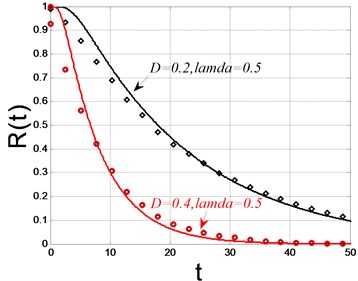
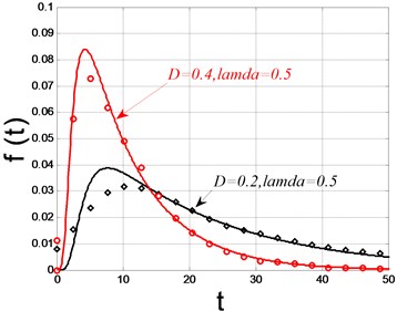
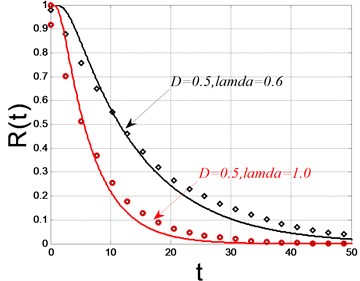
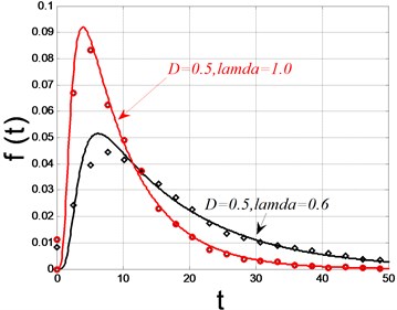
The critical value of the amplitude was set as 0.8, other parameters were set the same as those in the last section. The digital simulations were carried out, and the results were detailed in Fig. 5. The solid lines denote the theoretical solutions and the dots denote the digital simulations. Fig. 5(a) showed the reliability and Fig. 5(b) showed the probability density of the first passage failure with density 0.2, 0.4 and . It is clear that the reliability decreases with time and the larger the noise density is, the faster the reliability decreases. It is also obvious that larger noise density yields higher probability density of first passage failure. The influence of the time delay coefficient on the reliability was illustrated in Fig. 5(c) and Fig. 5(d). With noise density fixed as 0.5, time delay parameter was chosen as 0.6 and 1.0 respectively. The Fig. 5(c) and Fig. 5(d) showed that larger time delay parameter will result in faster decrease velocity of reliability and higher probability density of the first passage failure time. The numerical simulations are consistent with the theoretical prediction well enough, which means the drift coefficient and diffusion coefficient used in Eq. (25) are correct. Consequently, it is reasonable to believe that the stochastic averaging method we modified in this paper is accurate in calculating the drift coefficient and diffusion coefficient. The expression of the drift coefficient and diffusion coefficient is not very complex and the accuracy is acceptable.
Fig. 5The reliability function and the probability of fist passage failure time (solid lines: theoretical solutions; dots: digital simulations)
a)
b)
c)
d)
5. Conclusions
A modified stochastic averaging method dealing with colored noise excited oscillators is proposed in this paper, with the help of the He’s energy balance method the expression of the drift coefficient and diffusion coefficient are shorten significantly without weakening the accuracy too much. The amount of calculating has been reduced consequently. The Duffing-Rayleigh oscillator subject to colored noise excitation was taken as an example to verify the method. The probability of stationary responses of the amplitude and the joint probability of displacement and velocity are all studied. Furthermore, the reliability and the first passage failure are also studied. All the analytical approximations are consistent with the digital simulations.
References
-
Landau P. S., Stratonovich R. L. Theory of stochastic transitions of various systems between different states. Proceedings of Moscow University, Vol. 3, 1962, p. 33-45, (in Russian).
-
Khasminskii R. Z. On the behavior of a conservative system with small friction and small random noise. Journal of Applied Mathematics and Mechanics, Vol. 28, 1964, p. 1126-1130, (in Russian).
-
Zhu W. Q. Stochastic averaging of the energy envelope of nearly Lyapunov systems. Proceedings of the IUTAM Symposium on Random Vibrations and Reliability, Akademie, Berlin, 1983, p. 347-357.
-
Zhu W. Q., Lin Y. K. Stochastic averaging of energy envelope. Journal of Engineering Mechanics, Vol. 117, Issue 8, 1991, p. 1890-1905.
-
Red-Horse J. R., Spanos P. D. A generalization to stochastic averaging in random vibration. International Journal of Non-Linear Mechanics, Vol. 27, Issue 1, 1992, p. 85-101.
-
Cai G. Q. Random vibration of nonlinear systems under non-white excitations. Journal of Engineering Mechanics, Vol. 121, Issue 5, 1995, p. 637-639.
-
Dementberg M., Cai G. Q., Lin Y. K. Application of quasiconservative averaging to a non-linear system under non-white excitation. International Journal of Non-Linear Mechanics, Vol. 30, Issue 5, 1995, p. 677-685.
-
Cai G. Q., Lin Y. K., Xu W. Strongly Nonlinear System under Non-White Random Excitations. Book Series, Stochastic Structural Dynamics, Balkema, Rotterdam, 1999, p. 11-16.
-
Krenk S., Roberts J. B. Local similarity in nonlinear random vibration. Journal of Applied Mechanics, Vol. 66, Issue 1, 1999, p. 225-235.
-
Huang Z. L., Zhu W. Q. Stochastic averaging of quasi-integrable Hamiltonian systems under combined harmonic and white noise excitations. International Journal of Non-Linear Mechanics, Vol. 39, Issue 9, 2004, p. 1421-1434.
-
Zhu W. Q., Yang Y. Q. Stochastic averaging of quasi-nonintegrable-Hamiltonian systems. Journal of Applied Mechanics, Vol. 64, Issue 1, 1997, p. 157-164.
-
Zhu W. Q., Huang Z. L., Yang Y. Q. Stochastic averaging of quasi-integrable-Hamiltonian systems. Journal of Applied Mechanics, Vol. 64, Issue 4, 1997, p. 975-984.
-
Xu Z., Chung Y. K. Averaging method using generalized harmonic functions for strongly non-linear oscillators. Journal of Sound and Vibration, Vol. 174, Issue 4, 1994, p. 563-576.
-
Huang Z. L., Zhu W. Q. Stochastic averaging of strongly non-linear oscillators under combined harmonic and white-noise excitations. Journal of Sound and Vibration, Vol. 238, Issue 2, 2000, p. 233-256.
-
Zhu W. Q., Huang Z. L., Suzuki Y. Response and stability of strongly non-linear oscillators under wide-band random excitation. International Journal of Non-Linear Mechanics, Vol. 36, Issue 8, 2001, p. 1235-1250.
-
He J. H. Preliminary report on the energy balance for nonlinear oscillations. Mechanics Research Communications, Vol. 29, Issues 2-3, 2002, p. 107-111.
-
Davodi A. G., Ganji D. D., Azami R., et al. Application of improved amplitude-frequency formulation to nonlinear differential equation of motion equations. Modern Physics Letters. Vol. 23, Issue 28, 2009, p. 3427-3436.
-
Ganji S. S., Ganji D. D., Karimpour S. He’s energy balance and He’s variation methods for nonlinear oscillations in engineering. International Journal of Modern Physics B, Vol. 23, Issue 3, 2009, p. 461-471.
-
Mehdipour I., Ganji D. D., Mozaffari M. Applications of the energy balance method to nonlinear vibrating equations. Current Applied Physics, Vol. 10, Issue 1, 2010, p. 104-112.
-
Hui-Li Zhang. Periodic solutions for some strongly nonlinear oscillations by He’s energy balance method. Computers and Mathematics with Applications, Vol. 58, Issues 11-12, 2009, p. 2480-2485.
-
Vounesian Davood, Askari Hassan, Saadatnia Zia, et al. Frequency analysis of strongly nonlinear generalized Duffing oscillators using He’s frequency-amplitude formulation and He’s energy balance method. Computers and Mathematics with Applications, Vol. 59, Issue 9, 2010, p. 3222-3228.
-
Honeycutt Rebecca L. Stochastic Runge-Kutta algorithms. Part 2: colored noise. Physical Review A, Vol. 45, Issue 2, 1992, p. 604-610.
About this article

The authors gratefully acknowledge the support of the Natural Science Foundation of China (NSFC) through Grant Nos. 11402186 and 11302144 and the Tianjin Research Program of Application Foundation and Advanced Technology through Grant Nos. 14JCQNJC05600, 13JCYBJC17900, 14JCQNJC05300.
