Abstract
This paper discusses the portfolio optimization problem in an effective boundaries were drawn based on the efficient frontier portfolios which is analyzed using mean-variance model empirical method and simulated annealing algorithm. The conclusions show that drawing the efficient frontier based on simulated annealing algorithm is relatively accurate.
1. Introduction
Portfolio optimization problem is that multiple varieties of portfolio investment choices of investors formed by various securities products, such as stocks, bonds, etc., under certain constraints, to make the investment maximizing returns to investors. The purpose of the investment is to get the maximum benefit and bear minimal risk. In order to find a balance between expected return and risk of investment, Markowitz first put forward the securities portfolio theory, many scholars have studied based on the theory of portfolio optimization problems, such as the research based on the mean-VAR portfolio optimization problems using mean-VAR method, which proposed optimal portfolio model in the presence of transaction costs [1]. The others proposed venture capital portfolio optimization model, the use of agency theory to establish a venture capital portfolio optimization model. The optimal solution is given by the model number of items and the proportion of income distribution [2]. How to find the portfolio efficient frontier, there is no specific literature research relating to this issue. In addition to using traditional mean-variance efficient frontier model, we can also use the simulated annealing algorithm in the stochastic control theory to map out the portfolio efficient frontier. This article is based on two methods to draw the portfolio efficient frontier.
2. The mean-variance model’s efficient frontier
2.1. The concept of mean-variance model
Markowitz (1952) proposed a choice theory of portfolio which can be achieved under conditions of uncertainty [3]: mean-variance model methods. The basic idea of this method is as follows: the expected return of the portfolio is a weighted average of each of the assets constituting the portfolio rate of return to form for the weight ratio of the contribution of assets to the expected rate of return for each portfolio depends on its expected rate of return. Assuming assets 1, 2,…, on the market, the expected rate of return of asset is , the variance is , the covariance of asset and asset are (or the correlation coefficient is ), ( 1, 2,…, , 1, 2,…, ). The ratio of invested in asset is , 1, 2,…, .
Expected return for the portfolio is Eq. (1):
Multi-asset portfolio variance is Eq. (2):
Covariance is a statistical measure of the relationship between two random variables, it measures two random variables. The covariance assets can be expressed as Eq. (3):
Multi-asset Variance-covariance matrix is Eq. (4):
2.2. The empirical analysis
Based on a large number of transactions recorded on a stock exchange regarding to 20 stocks over six months, we calculated the covariance matrix and average earnings about 20 stocks in the statistical analysis software R language. The average yield in the form of drawing scatter plot was shown in Fig. 1. The average expected rate of return about 20 stocks shows scattered in the figure.
Fig. 1The expected rate of return about 20 stocks
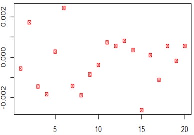
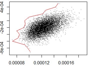
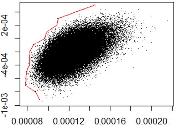
Fig. 2Simulation of 10,000 and 100,000 times of the portfolio’s efficient frontier
a)
b)
The use of the R statistical software can draw the portfolio’s efficient frontier about 20 stocks. According to the principle of mean-variance model, randomly simulate 10,000 and 100,000 times the weight of the portfolio, the entire portfolio of stippling was drawn in the mean variogram. Select the lowest point of the risk under each expected return that is standard deviation of the minimum point drawn the efficient frontier curve, as shown in Fig. 2. As can be seen from the figure, the implementation process of this method is relatively simple and requires a lot of simulation to get a relatively effective result, and there are some differences between the 10,000 and 100,000 times of the efficient frontier simulation results, it is not very accurate.
3. Based on the efficient frontier of the simulated annealing algorithm
3.1. The idea of the simulated annealing algorithm
Simulated annealing algorithm originated in physical annealing process, simulated annealing algorithm was first proposed by Metropolis (1953), and Kirkpatrick (1983) applied it to combinatorial optimization [4]. The principle can be expressed as: annealing mimic natural phenomenon obtained by the similarity of the physical annealing process of the solid material in the general optimization problem. Starting from a certain initial temperature accompanied by declining temperatures, combine with the probability of the sudden jump in the solution space stochastic characteristics to find the global optimal solution. It mimics the physical annealing heating isothermal and cooling process, at a certain temperature, the search randomly change from one state to another state, with the lowest temperature until the temperature drops, the search process to find the global optimal solution. Mathematical ideas can be expressed as follows.
At temperature , the molecule stays in state satisfy Boltzmann probability distribution, as shown in Eqs. (5) (6):
At the same temperature the selected two energy , there is Eq. (7):
The main steps of simulated annealing algorithm can be expressed as follows [5]:
Initialization: Given the initial temperature t=t0;
Randomly generated initial states=s0;
k=0;
Repeat
Repeat
Generate new state: sj=Generate(s);
If min {1,exp [-(C(sj)-C(s))/tk]}>=random[0,1] s=sj;
Until meet the sampling stability criteria;
Return temperature tk+1=update(tk) and make k=k+1;
Until Algorithm terminates meet the criteria;
The output of the algorithm search results.
3.2. The empirical analysis
Based on the basic idea of simulated annealing method, it needs to determine the initial temperature and internal cycles, these two parameters are the most important parameters directly determine the effect of the number of cycles and optimize the algorithm. If the initial temperature is set too low, the temperature drop less times, leading to the possibility of searching the global optimum to be less likely. On the contrary, if the initial temperature is set too high, the temperature drop more times, the possibility to search the global optimum is greater. However the increase will reduce the number of iterations of the feasibility and effectiveness of the algorithm, therefore it need several attempts to determine the efficient frontier of simulated annealing method to select the most suitable parameter control cycles and results.
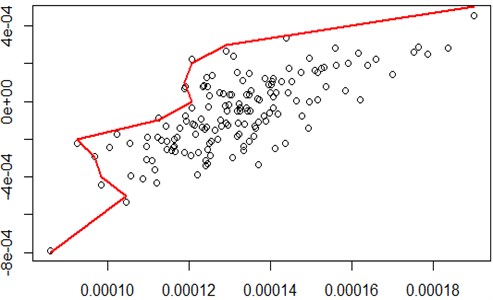
When the initial temperature is set to 10000, inner cycles is set to 10, using R statistical software to draw the effective boundaries was shown in Fig. 3. It can be seen from the figure, the points of 20 stocks portfolio is dispersed, the number of less cycles makes efficient frontier not obvious.
Fig. 3Initial temperature of 10000, 10 cycles of simulated annealing method for the efficient frontier
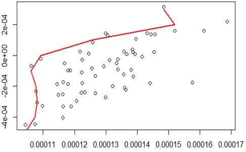
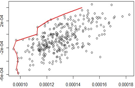
When the initial temperature increase to 100000, the number of cycles 50, the points of 20 stocks portfolio is more concentrated stock, optimized results were better. The effective boundary was shown in Fig. 4.
Fig. 4Initial temperature of 100 000, 50 cycles of simulated annealing method for the efficient frontier (to optimize the efficient frontier)
When the initial temperature is up to 1 million, the number of cycles 100, the points of 20 stocks portfolio concentration is not very good, there is no effective border compared to Fig. 4, as shown in Fig. 5, therefore, according to 20 stocks portfolio optimization effective border, the efficient frontier select best shown in Fig. 4.
Fig. 5Initial temperature of one million, 100 cycles of simulated annealing method for the efficient frontier
4. Conclusions
Based on the two methods above, we can draw the efficient frontier of the portfolio optimization problem. From the effects of the empirical point of view, the use of mean-variance model approach to map out effective border is relatively simple, the results can be get based on a number of simulation. Anyway this article is based on a simulation demo of 20 stocks transactions, if the number of portfolio is too much, for example 1000 stock situation, using this method is difficult to get effective results, and requires a lot of simulation, it is easily lead to computer crashes. However, this method is most commonly used method as a research portfolio optimization problems, it has been widely used in reality. Based on simulated annealing algorithm to map out effective border portfolio is relatively accurately, and in a relatively faster computing speed. This paper was based on this method of an empirical model does also found a relatively precise and effective border graphics.
References
-
Rongxi Min, Wu Dandan, Zhang Kuiting Optimal portfolio based on the average – VAR model. Mathematical Statistics and Management, Vol. 25, 2005.
-
Zhang Xinli, Yang De, Wang Qing Jiang Model of optimizing portfolio risk capital. Economic Mathematics, Vol. 4, 2005.
-
Elton Edwin J., Gruber Martin J., Brow Stephen J., Goetmann William N. Modern Portfolio Theory and Investment Analysis, 7 Edition. 2008, p. 28-42.
-
Zhu Hao-dong, Chung Yong An improved simulated annealing algorithm. Computer Technology and Development, Vol. 19, 2009.
-
Chi Yu, Zhang Fei, Wang Zhenglin Data Analysis: R Language Practice. Beijing Electronic Industry Press, 2014, p. 289-297.
About this article
