Vibration and stability of internally damped rotating composite Timoshenko shaft

Ren, Yongsheng; Zhang, Yuhuan; Zhang, Xingqi

Journal of Vibroengineering

Browse Journal

Submit article

Published: 30 December 2015

Check for updates

Vibration and stability of internally damped rotating composite Timoshenko shaft

Yongsheng Ren¹

Yuhuan Zhang²

Xingqi Zhang³

^{1, 2, 3}College of Mechanical and Electronic Engineering, Shandong University of Science and Technology, Qingdao, 266590, China

Corresponding Author:

Yongsheng Ren

Cite the article Download PDF

Downloads 1437

WoS Core Citations 7

Abstract

The mechanical model for the dynamic behavior of an internally damped rotating composite shaft is derived using a refined variational asymptotic method and the principle of virtual work. The composite shaft is considered as an anisotropic thin-walled Timoshenko beam. The internal damping of composite shaft is modelled by adopting the multi-scale damping analysis method. Galerkin’s method is employed to discretize and solve the equations of motion. The effect of design parameters including fiber orientation, length aspect ratio, stacking sequences and boundary conditions on the free vibration and stability of composite shaft is investigated.

1. Introduction

The rotating composite shafts are now used widely in many application areas involving the rotating machinery systems. In the last few years, there exists numerous researches related to predicting natural frequencies and critical speeds of composite shaft [1-9]. As rotating speed is above the first critical speed, the effect of internal damping on the dynamic stability of rotating shaft becomes increasingly important. The sources of internal damping in rotating shaft can be due to material damping or friction. Composite shafts have higher material damping than conventional metallic shafts. Therefore, accurate prediction of effects of composite internal damping on the dynamical behavior of rotating composite shafts are necessary for improving performance of the shaft system. So far, only less work seems to have been reported towards the stability analysis, particularly effects of internal damping on the stability of a rotating composite shaft [10-13]. Singh and Gupta [10] introduced discrete viscous damping coefficients to account for effect of internal damping. In a similar approach, dynamic instability analysis of composite shaft has been performed by Kim et al. [11], Mazzei and Scott [12] as well as Montagnier and Hochard [13]. In above cases, internal damping terms were included simply in equations of motion of rotating shaft, no internal damping modeling has been described. Sino et al. [14] investigated the stability of an internally damped rotating composite shaft. Internal damping was introduced by the complex constitutive relation of a viscoelastic composite. The shaft was modelled by finite element method. However, only the elastic coupling effects induced by symmetrical stacking are taken into account in their mode. Ren et al. [15] presented the dynamical analysis of rotating composite thin-walled shafts with internal damping based on variational asymptotically method (VAM) [16], which is able to represent the cross-sectional warping and various elastic couplings by symmetrical or unsymmetrical stacking. Internal damping of the shaft is introduced via the multi-scale damping mechanics [17] but transverse shear deformation has not been taken into account in the model.

In the present work, a refined VAM composite thin-walled beam theory which incorporates the effect of transverse shear deformation is used for the dynamical analysis of rotating composite thin-walled shafts with internal damping. The equations of motion of the rotating Timoshenko composite shafts are derived by the principle of virtual work. The internal damping of composite shaft is modelled based on the multi-scale damping mechanics [17]. Galerkin’s method is applied to discretize and solve the governing equations. The critical rotating speeds and instability thresholds are obtained through numerical simulations. The effects of fiber orientation, length aspect ratio, stacking sequences and boundary conditions are assessed. The validity of the model is proved by comparing the results with those in literature and convergence examination.

2. Theoretical formulations and numerical method

2.1. The displacement and strain

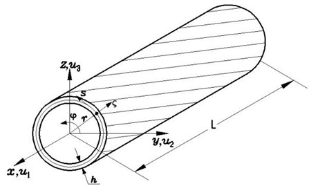
The symbols $L$ , $h$ and $r$ represent the length, wall thickness and radius of the shaft, respectively. The inertial reference system $(X, Y, Z)$ and rotating reference system $(x, y, z)$ will be used for describing the motion of the shaft. The ( $I, J, K)$ and $(i, j, k)$ are the unit vectors with respect to the reference system $(X, Y, Z)$ and $(x, y, z)$ , respectively. In addition, a curvilinear coordinate system $(ς, s, x)$ is also used, where and $s$ is the circumferential coordinate measured along the tangent to the middle surface, whereas $ς$ is measured along the normal to the middle surface.

The displacement field incorporating shear deformation in the local frame denoted $(x, s, ξ)$ is assumed in the form [9]:

1

u_{1} (x, y, z, t) = U_{1} (x, t) - y (s) θ_{y} (x, t) - z (s) θ_{z} (x, t) + g (s, x, t),

u_{2} (x, y, z, t) = U_{2} (x, t) - z ϕ (x, t), u_{3} (x, y, z, t) = U_{3} (x, t) + y ϕ (x, t),

where, $U_{1} (x, t)$ , $U_{2} (x, t)$ , $U_{3} (x, t)$ denote the average displacements along the $x$ , $y$ and $z$ -axis, while $ϕ (x, t)$ , $θ_{y} (x, t)$ , $θ_{z} (x, t)$ denote the twist angles about the $x$ -axis and rotations about the $y$ and $z$ -axis, respectively.

The warping functions $g (s, x, t)$ can be assumed as follows:

2

g (s, x, t) = G (s) ϕ^{'} (x, t) + g_{1} (s) U_{1}^{'} (x, t) + g_{2} (s) θ_{y}^{'} (x, t) + g_{3} (s) θ_{z}^{'} (x, t) .

In the above equation, the functions $g_{1} (s)$ , $g_{2} (s)$ , $g_{3} (s)$ , $G (s)$ associated with physical behavior for the axial strain, the bending curvatures, and the torsion twist rate, respectively. The primes in Eq. (2) denote differentiation with respect to $x$ .

In Eqs. (1) and (2), the expressions of $θ_{y} (x, t)$ , $θ_{z} (x, t)$ are in the form as follows:

3

θ_{y} (x, t) = U_{2}^{'} (x, t) - 2 γ_{z 1},

θ_{z} (x, t) = U_{3}^{'} (x, t) - 2 γ_{y 1} .

The strain of the composite shaft can be expressed as [9]:

4

γ_{11} = U_{1}^{'} (x, t) - y θ_{y}^{'} (x, t) - z θ_{z}^{'} (x, t),

2 γ_{1 s} = \frac{d g}{d s} + r_{n} ϕ^{'} + (U_{2}^{'} (x, t) - θ_{y} (x, t)) \frac{d y}{d s} + (U_{3}^{'} (x, t) - θ_{z} (x, t)) \frac{d z}{d s},

2 γ_{x ξ} = (U_{2}^{'} (x, t) - θ_{y} (x, t)) \frac{d z}{d s} - (U_{3}^{'} (x, t) - θ_{z} (x, t)) \frac{d y}{d s} .

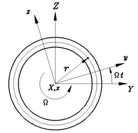
The position vector of an arbitrary point on the cross-section of the deformed shaft is $R = (y + u_{2}) i + (z + u_{3}) j + (x + u_{1}) k$ . Here, $i$ , $j$ , $k$ are unit vectors of the coordinate systems $(x, y, z)$ . By taking the time derivatives of unit vectors and adopting the assumption of constant rate $Ω,$ the velocity and acceleration vector of an arbitrary point are:

\dot{R} = [{\dot{u}}_{2} - Ω (z + u_{3})] i + [{\dot{u}}_{3} + Ω (y + u_{2})] j + {\dot{u}}_{1} k,

and

\ddot{R} = [{\ddot{u}}_{2} - 2 Ω {\dot{u}}_{3} - Ω^{2} (y + u_{2})] i + [{\ddot{u}}_{3} + 2 Ω \dot{u_{2}} - Ω^{2} (z + u_{3})] j + {\ddot{u}}_{1} k,

respectively.

Fig. 1Geometry and coordinate systems of composite thin-walled shaft

2.2. Equations of motion

The equations of motion of the shaft can be described by a variational form:

5

\int_{0}^{l} (δ U_{s} - δ T_{s} + δ W_{s}) d x = 0,

where $δ U_{s}$ , $δ T_{s}$ and $δ W_{s}$ are the variation of the strain energy, kinetic energy and the dissipated energy of cross-section, respectively.

2.2.1. The strain energy and dissipated energy

The strain energy and dissipated energy of composite shaft can be described by multi-scale modelling for each composite ply, for the laminate, for cross-section and eventually for the complete shaft.

2.2.1.1. Equivalent cross-section stiffness matrix

The strain energy density of a composite ply can be expressed as:

6

φ = \frac{1}{2} (σ_{11} γ_{11} + σ_{s s} γ_{s s} + 2 τ_{1 s} γ_{1 s} + 2 τ_{ξ 1} γ_{ξ 1} + 2 τ_{ξ s} γ_{ξ s}) .

The stress-strain relation is written as:

7

[\begin{matrix} σ_{11} \\ σ_{s s} \\ τ_{1 s} \end{matrix}] = [\begin{matrix} {\bar{Q}}_{11} & {\bar{Q}}_{12} & {\bar{Q}}_{16} \\ {\bar{Q}}_{12} & {\bar{Q}}_{22} & {\bar{Q}}_{26} \\ {\bar{Q}}_{16} & {\bar{Q}}_{26} & {\bar{Q}}_{66} \end{matrix}] [\begin{matrix} γ_{11} \\ γ_{s s} \\ 2 γ_{1 s} \end{matrix}], [\begin{matrix} τ_{ξ 1} \\ τ_{ξ s} \end{matrix}] = [\begin{matrix} κ {\bar{Q}}_{44} & κ {\bar{Q}}_{45} \\ κ {\bar{Q}}_{45} & κ {\bar{Q}}_{55} \end{matrix}] [\begin{matrix} 2 γ_{ξ 1} \\ 2 γ_{ξ s} \end{matrix}],

where, $[{\bar{Q}}_{i j}]$ is equivalent off-axis stiffness matrix of a composite ply with respect to the system $o s x ς$ , $κ = 1 / (2 - G_{12} ν_{12} / E_{1})$ is a Timoshenko shear coefficient [18].

Substituting Eq.(7) into (6) and integrate over the thickness $ξ$ to obtain the strain energy of the laminate as following:

8

2 \hat{φ} = A_{11} γ_{11}^{2} + A_{22} γ_{s s}^{2} + 4 A_{66} γ_{1 s}^{2} + 2 A_{12} γ_{11} γ_{s s} + 4 A_{16} γ_{11} γ_{1 s} + 4 A_{26} γ_{1 s} γ_{s s} + 4 A_{44} γ_{ξ 1}^{2}

+ 4 A_{55} γ_{ξ s}^{2} + 8 A_{45} γ_{ξ 1} γ_{ξ s},

where the laminate in-plane stiffnesses are:

9

A_{i j} = \int_{- h / 2}^{h / 2} {\bar{Q}}_{i j} d ξ = 2 \sum_{k = 1}^{N / 2} {\bar{Q}}_{i j}^{k} (h_{k} - h_{k - 1}), (i, j = 1, 2, 6),

A_{i j} = \int_{- h / 2}^{h / 2} {\bar{Q}}_{i j} d ξ = 2 \sum_{k = 1}^{N / 2} {\bar{Q}}_{i j}^{k} (h_{k} - h_{k - 1}), (i, j = 4, 5) .

For the case of no internal pressure acting on the shaft, Eq. (8) can be simplified by using free hoop stress resultants assumption ( $N_{s s} = 0$ , $N_{ξ s} = 0$ ) and then integrating the resulted expression around the cross-sectional midline to get the strain energy of cross-section in terms of the generalized displacements and the equivalent cross-section stiffness matrix, as follows:

10

{\hat{U}}_{s} = \frac{1}{2} {\{δ\}}^{T} K \{δ\},

where ${\{δ\}}^{T} = \{U_{1}^{'} ϕ^{'} θ_{z}^{'} θ_{y}^{'} U_{2}^{'} - θ_{y} U_{3}^{'} - θ_{z}\},$ $K$ is 6×6 symmetric stiffness matrix, the coefficients $k_{i j}$ ( $i$ , $j =$ 1, 2, …, 4) represent the stiffness, as described in [16] for the case of an non-shearable thin-walled beam, while the transverse shear deformation contribution to the stiffness coefficients is represented by the new terms $k_{i j}$ ( $i =$ 1, 2,…, 6; $j =$ 5, 6), $k_{j i}$ ( $i =$ 1, 2, 3, 4; $j =$ 5, 6) [9].

Injecting a Timoshenko shear coefficient $κ$ , the new stiffness coefficient terms $k_{i j}$ ( $i =$ 1, 2,…, 6; $j =$ 5, 6), $k_{j i}$ ( $i =$ 1, 2,…,4; $j =$ 5, 6) can be expressed as:

11

k_{15} = \frac{1}{2} κ \oint_{Γ}^{} B \frac{d y}{d s} d s, k_{16} = \frac{1}{2} κ \oint_{Γ}^{} B \frac{d z}{d s} d s, k_{25} = \frac{1}{4} κ \oint_{Γ}^{} r_{n} C \frac{d y}{d s} d s,

k_{26} = \frac{1}{4} κ \oint_{Γ}^{} r_{n} C \frac{d z}{d s} d s, k_{35} = - \frac{1}{2} κ \oint_{Γ}^{} B z \frac{d y}{d s} d s, k_{36} = - \frac{1}{2} κ \oint_{Γ}^{} B z \frac{d z}{d s} d s,

k_{45} = - \frac{1}{2} κ \oint_{Γ}^{} B y \frac{d y}{d s} d s, k_{46} = - \frac{1}{2} κ \oint_{Γ}^{} B y \frac{d z}{d s} d s,

k_{55} = κ \oint_{Γ}^{} [\frac{1}{4} C {(\frac{d y}{d s})}^{2} + D {(\frac{d z}{d s})}^{2}] d s, k_{56} = κ \oint_{Γ}^{} (\frac{1}{4} C - D) \frac{d y}{d s} \frac{d z}{d s} d s,

k_{66} = κ \oint_{Γ}^{} [\frac{1}{4} C {(\frac{d z}{d s})}^{2} + D {(\frac{d y}{d s})}^{2}] d s,

where:

12

A (s) = A_{11} - \frac{A_{12}^{2}}{A_{22}}, B (s) = 2 [A_{16} - \frac{A_{12} A_{26}}{A_{22}}], C (s) = 4 [A_{66} - \frac{A_{26}^{2}}{A_{22}}],

D (s) = (A_{44} - \frac{A_{45}^{2}}{A_{55}}), A_{i j} = \sum_{k = 1}^{N} {\bar{Q}}_{i j}^{(k)} (z_{k} - z_{k - 1}), (i, j = 1, 2, 6; i j = 4, 5) .

In above equations, the variables $A (s)$ , $B (s)$ , $C (s)$ and $D (s)$ represent the reduced axial, coupling, and shear stiffness of cross-section, respectively. The variables $A (s)$ , $B (s)$ , $C (s)$ correspond to the stiffness coefficients for non-shearable thin-walled beam [16]. The new variable $D (s)$ results from the transverse shear deformation.

By performing the integral along the length $L$ , the strain energy of the shaft can be expressed as following:

13

U_{s} = \int_{0}^{L} {\hat{U}}_{s} d x = \frac{1}{2} \int_{0}^{L} {\{δ\}}^{T} K \{δ\} d x .

2.2.1.2. Equivalent cross-section damping matrix

The dissipated energy density of a composite ply can be written as:

14

Δ φ = \frac{1}{2} (σ_{11} η_{11} γ_{11} + σ_{s s} η_{s s} γ_{s s} + 2 τ_{1 s} η_{1 s} γ_{1 s} + 2 τ_{ξ 1} η_{ξ 1} γ_{ξ 1} + 2 τ_{ξ s} η_{ξ s} γ_{ξ s}),

where $η_{i j}$ are off-axis damping coefficients of a composite ply.

The dissipated energy of the laminate has following form:

15

2 Δ \hat{φ} = A_{d 11} γ_{11}^{2} + A_{d 22} γ_{s s}^{2} + 4 A_{d 66} γ_{1 s}^{2} + (A_{d 12} + A_{d 21}) γ_{11} γ_{s s} + 2 (A_{d 16} + A_{d 61}) γ_{11} γ_{1 s}

+ 2 (A_{d 26} + A_{d 62}) γ_{1 s} γ_{s s} + 4 A_{d 44} γ_{ξ 1}^{2} + 4 A_{d 55} γ_{ξ s}^{2} + 4 (A_{d 45} + A_{d 54}) γ_{ξ 1} γ_{ξ s},

where the laminate dampings in-plane are:

16

A_{d i j} = \int_{- h / 2}^{h / 2} η_{i l} {\bar{Q}}_{l j} d ξ = 2 \sum_{k = 1}^{N / 2} η_{i l}^{k} {\bar{Q}}_{l j}^{k} (h_{k} - h_{k - 1}), (i, j, l = 1, 2, 6),

A_{d i j} = \int_{- h / 2}^{h / 2} η_{i l} {\bar{Q}}_{l j} d ξ = 2 \sum_{k = 1}^{N / 2} η_{i l}^{k} {\bar{Q}}_{l j}^{k} (h_{k} - h_{k - 1}), (i, j, l = 4, 5),

where $[η_{i j}] = {[R]}^{T} [η_{l}] [R]$ , $[R]$ is transformation matrix. $[η_{l}] = d i a g (η_{l 1}, η_{l 2}, η_{l 4}, η_{l 5}, η_{l 6})$ is the on-axis damping matrix within a ply.

Similar to the derivation of Eq. (10) for the strain energy of cross-section, the dissipated energy of cross-section can be obtained in terms of generalized displacements and the equivalent cross-section damping matrix as follows:

17

{\hat{W}}_{s} = \frac{1}{2} {\{δ\}}^{T} C \{δ\},

where $[C]$ is 6×6 symmetric damping matrix. The formulation of its components $c_{i j}$ is analogous to stiffness components $k_{i j}$ as shown in Eqs. (10) and (11), but the terms $A$ , $B$ , $C$ and $D$ in Eqs. (10) and (11) should be replaced by the terms $A_{d}$ , $B_{d}$ , $C_{d}$ and $D_{d}$ , respectively.

The variables $A_{d}$ , $B_{d}$ , $C_{d}$ and $D_{d}$ are given by:

18

A_{d} (s) = A_{d 11} + (\frac{A_{12}^{2}}{A_{22}^{2}}) A_{d 22} - (\frac{A_{12}}{A_{22}}) (A_{d 12} + A_{d 21}),

B_{d} (s) = A_{d 16} + A_{d 61} + 2 (\frac{A_{12} A_{26}}{A_{22}^{2}}) A_{d 22} - (\frac{A_{26}}{A_{22}}) (A_{d 12} + A_{d 21}) - (\frac{A_{12}}{A_{22}}) (A_{d 26} + A_{d 62}),

C_{d} (s) = 4 [A_{d 66} + (\frac{A_{26}^{2}}{A_{22}^{2}}) A_{d 22} - (\frac{A_{26}}{A_{22}}) (A_{d 26} + A_{d 62})],

D_{d} (s) = 4 [A_{d 44} + (\frac{A_{45}^{2}}{A_{55}^{2}}) A_{d 55} - (\frac{A_{45}}{A_{55}}) (A_{d 45} + A_{d 54})] .

The dissipated energy of the shaft can be expressed as following:

19

W_{s} = \int_{0}^{L} {\hat{W}}_{s} d s = \frac{1}{2} \int_{0}^{L} {\{δ\}}^{T} C \{δ\} d x .

2.2.2. The kinetic energy

The kinetic energy of the cross-section of rotating shaft is:

20

T_{s} = - \oint \int_{- h / 2}^{h / 2} R^{T} [d i a g (ρ)] \ddot{R} d ξ d s,

where $[d i a g (ρ)]$ is a diagonal matrix with components equal to the mass density $ρ$ of a ply.

Substituting the expressions of $R$ and $\ddot{R}$ into Eq. (20), the kinetic energy of cross-section can be obtained as:

21

{\hat{T}}_{s} = - (I_{1} δ U_{1} + I_{2} δ U_{2} + I_{3} δ U_{3} + I_{4} δ θ_{y} + I_{5} δ θ_{z} + I_{6} δ ϕ),

where:

22

I_{1} = b_{1} {\ddot{U}}_{1} - b_{2} {\ddot{θ}}_{y} - b_{3} {\ddot{θ}}_{z},

I_{2} = b_{1} ({\ddot{U}}_{2} - 2 Ω {\dot{U}}_{3} - Ω^{2} U_{2}) - b_{2} (2 Ω \dot{ϕ} + Ω^{2}) - b_{3} (\ddot{ϕ} - Ω^{2} ϕ),

I_{3} = b_{1} ({\ddot{U}}_{3} + 2 Ω {\dot{U}}_{2} - Ω^{2} U_{3}) + b_{2} (\ddot{ϕ} - Ω^{2} ϕ) - b_{3} (2 Ω \dot{ϕ} + Ω^{2}),

I_{4} = b_{2} {\ddot{U}}_{1} - b_{4} {\ddot{θ}}_{y} - b_{6} {\ddot{θ}}_{z}, I_{5} = b_{3} {\ddot{U}}_{3} - b_{6} {\ddot{θ}}_{y} - b_{5} {\ddot{θ}}_{z},

I_{6} = b_{2} ({\ddot{U}}_{3} + 2 Ω {\dot{U}}_{2} - Ω^{2} U_{3}) + (b_{4} + b_{5}) (\ddot{ϕ} - Ω^{2} ϕ) - b_{3} ({\ddot{U}}_{2} - 2 Ω {\dot{U}}_{3} - Ω^{2} U_{2}),

b_{1} = \oint ρ h (s) d s, b_{2} = \oint ρ y h (s) d s, b_{3} = \oint ρ z h (s) d s,

b_{4} = \oint ρ y^{2} h (s) d s, b_{5} = \oint ρ z^{2} h (s) d s, b_{6} = \oint ρ y z h (s) d s .

The kinetic energy of the shaft can be expressed as following:

23

T_{s} = \int_{0}^{L} {\hat{T}}_{s} d x = - \int_{0}^{L} (I_{1} δ U_{1} + I_{2} δ U_{2} + I_{3} δ U_{3} + I_{4} δ θ_{y} + I_{5} δ θ_{z} + I_{6} δ ϕ) d x .

The approximate solutions are assumed for $U_{1} (x, t)$ , $U_{2} (x, t)$ , $U_{3} (x, t)$ , $θ_{y} (x, t)$ , $θ_{z} (x, t)$ and $ϕ (x, t)$ in the form:

24

U_{1} (x, t) = \sum_{j = 1}^{N} U_{1 j} β_{j} (x) e^{i λ t}, U_{2} (x, t) = \sum_{j = 1}^{N} U_{2 j} α_{j} (x) e^{i λ t},

U_{3} (x, t) = \sum_{j = 1}^{N} U_{3 j} α_{j} (x) e^{i λ t}, θ_{y} (x, t) = \sum_{j = 1}^{N} Θ_{y j} ψ_{j} (x) e^{i λ t},

θ_{z} (x, t) = \sum_{j = 1}^{N} Θ_{z j} ψ_{j} (x) e^{i λ t}, ϕ (x, t) = \sum_{j = 1}^{N} Φ_{j} θ_{j} (x) e^{i λ t},

where $β_{j} (x)$ , $α_{j} (x)$ , $ψ_{j} (x)$ and $θ_{j} (x)$ represent mode shape functions. These functions satisfy the geometric boundary conditions at $x = 0$ and $x = L$ , $λ$ is complex eigenvalues of the system, $U_{1 j}$ , $U_{2 j}$ , $U_{3 j}$ , $Θ_{y j}$ , $Θ_{z j}$ and $Φ_{j}$ are undetermined constants, $i = \sqrt{- 1}$ .

Substituting Eq. (24) into the energy expressions (13), (19), (23) and (5), and using Galerkin method, one obtains the motion equations in matrix form:

25

{\{δ U\}}^{T} (- λ^{2} [M] + i λ [G] + i λ [C] + [K_{1}] + [K_{Ω}]) \{U\} = 0,

where ${\{U\}}^{T} = (\dots U_{1 j} \dots U_{2 j} \dots U_{3 j} \dots Θ_{y j} \dots Θ_{z j} \dots Φ_{j} \dots)$ is a constant vector; $[M]$ the mass matrix; $[G]$ the gyroscopic matrix, $[C]$ the damping matrix, $[K]$ the stiffness matrix, $[K_{Ω}]$ the stiffness matrix which depends on the rotational speed $Ω$ . The detailed expressions of these matrices are follows:

26

M = [\begin{matrix} b_{1} B_{i j} & 0 & 0 & 0 & 0 & 0 \\ 0 & b_{1} E_{i j} & 0 & 0 & 0 & 0 \\ 0 & 0 & b_{1} E_{i j} & 0 & 0 & 0 \\ 0 & 0 & 0 & - b_{4} F_{i j} & 0 & 0 \\ 0 & 0 & 0 & 0 & - b_{5} F_{i j} & 0 \\ 0 & 0 & 0 & 0 & 0 & (b_{4} + b_{5}) G_{i j} \end{matrix}],

27

K_{1} = [\begin{matrix} - k_{11} N_{i j} & 0 & 0 & 0 & 0 & - k_{12} D_{i j} \\ 0 & - k_{55} I_{i j} & 0 & k_{55} J_{i j} & - k_{35} K_{i j} & 0 \\ 0 & 0 & - k_{66} I_{i j} & - k_{46} K_{i j} & k_{66} J_{i j} & 0 \\ 0 & - k_{55} O_{i j} & - k_{46} P_{i j} & - k_{44} Q_{i j} + k_{55} F_{i j} & 0 & 0 \\ 0 & - k_{35} P_{i j} & - k_{66} O_{i j} & 0 & - k_{33} Q_{i j} + k_{66} F_{i j} & 0 \\ - k_{12} H_{i j} & 0 & 0 & 0 & 0 & - k_{22} L_{i j} \end{matrix}],

28

[Κ_{Ω}] = [\begin{matrix} 0 & 0 & 0 & 0 & 0 & 0 \\ 0 & - b_{1} Ω^{2} E_{i j} & 0 & 0 & 0 & 0 \\ 0 & 0 & - b_{1} Ω^{2} E_{i j} & 0 & 0 & 0 \\ 0 & 0 & 0 & 0 & 0 & 0 \\ 0 & 0 & 0 & 0 & 0 & 0 \\ 0 & 0 & 0 & 0 & 0 & - (b_{4} + b_{5}) Ω^{2} G_{i j} \end{matrix}],

29

[G] = [\begin{matrix} 0 & 0 & 0 & 0 & 0 & 0 \\ 0 & 0 & - 2 Ω b_{1} E_{i j} & 0 & 0 & 0 \\ 0 & 2 Ω b_{1} E_{i j} & 0 & 0 & 0 & 0 \\ 0 & 0 & 0 & 0 & 0 & 0 \\ 0 & 0 & 0 & 0 & 0 & 0 \\ 0 & 0 & 0 & 0 & 0 & 0 \end{matrix}],

30

C = [\begin{matrix} - c_{11} N_{i j} & 0 & 0 & 0 & 0 & - c_{12} D_{i j} \\ 0 & - c_{55} I_{i j} & 0 & c_{55} J_{i j} & - c_{35} K_{i j} & 0 \\ 0 & 0 & - c_{66} I_{i j} & - c_{46} K_{i j} & c_{66} J_{i j} & 0 \\ 0 & - c_{55} O_{i j} & - c_{46} P_{i j} & - c_{44} Q_{i j} + c_{55} F_{i j} & 0 & 0 \\ 0 & - c_{35} P_{i j} & - c_{66} O_{i j} & 0 & - c_{33} Q_{i j} + c_{66} F_{i j} & 0 \\ - c_{12} H_{i j} & 0 & 0 & 0 & 0 & - c_{22} L_{i j} \end{matrix}],

where:

31

E_{i j} = \int_{0}^{L} α_{i} α_{j} d x, F_{i j} = \int_{0}^{L} ψ_{i} ψ_{j} d x, I_{i j} = \int_{0}^{L} α_{i} α_{j}^{''} d x, J_{i j} = \int_{0}^{L} α_{i} ψ_{j}^{'} d x,

K_{i j} = \int_{0}^{L} α_{i} ψ_{j}^{''} d x, O_{i j} = \int_{0}^{L} ψ_{i} α_{j}^{'} d x, P_{i j} = \int_{0}^{L} ψ_{i} α_{j}^{''} d x, Q_{i j} = \int_{0}^{L} ψ_{i} ψ_{j}^{''} d x,

B_{i j} = \int_{0}^{L} β_{i} β_{j} d x, N_{i j} = \int_{0}^{L} β_{i} β_{j}^{''} d x, D_{i j} = \int_{0}^{L} β_{i} θ_{j}^{''} d x, G_{i j} = \int_{0}^{L} θ_{i} θ_{j} d x,

H_{i j} = \int_{0}^{L} θ_{i} β_{j}^{''} d x, L_{i j} = \int_{0}^{L} θ_{i} θ_{j}^{''} d x, (i, j = 1, \dots, N) .

From Eq. (25), one can obtain the following complex eigenvalue problem:

32

d e t \{- λ^{2} [M] + i λ ([G] + [C]) + [K]\} = 0 .

The complex eigenvalue $λ$ of Eq.(32) can be written as:

33

λ = σ + i ω .

The imaginary part $ω$ and the real part $σ$ of $λ$ give the damping natural frequency and the decay, respectively. If $σ$ is negative, the amplitude decays in time and the shaft has a stable behavior because the whirl motion tends to reduce its amplitude. On the other hand, if $σ$ is positive, the motion is unstable with the amplitude growing exponentially in time.

It should be emphasized that the equation (25) is obtained using the rotating reference system $(x, y, z)$ . Besides, when the ply angle distribution is a CUS (Circumferentially Uniform Stiffness) configuration [20], Eq. (25) can be decoupled into the flapping bending-sweeping bending equation and extension-twist equation. This paper will address the flapping bending-sweeping bending coupling and present all numerical results with reference to the rotating reference system. For simplicity, the resulting flapping bending-sweeping bending equation are not presented.

3. Numerical results

The natural frequency and modal damping of thin-walled beam with circular and box sections are predicted and shown in Table 1 and 2. The numerical results of present model are compared with those using shear beam finite element model [20] and non-shearable beam model [17]. As can been seen, the present model shows good agreement with those found in the literature.

The numerical calculations are performed by considering the composite shaft whose elastic characteristics are listed in Table 3. The shaft has circular cross-section of mean diameter $d =$ 0.352 m. Ply thickness is 0.000635 m, and the wall has 16 layers. The material properties of each ply are listed in Table 3.

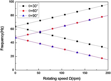
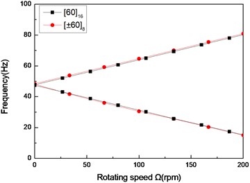
Figs. 2 show the first three natural frequencies vs. rotating speed for simply supported shear shaft and for various ply angles. From these figures it can be seen that when rotating speed equals to zero a single non-rotating natural frequency is obtained. As the rotating speed is increased, due to the gyroscopic effect, the natural frequencies ‘split’ into the upper and lower frequency branches. The upper frequency branch is associated with the forward whirling motion. Similarly, lower frequency branch is associated with the backward whirling motion. The minimum rotating speed at which the lower frequency becomes zero is referred to as the critical rotating speed. It is also seen that with the decrease of ply angle the non-rotating natural frequencies increase. This is because the closer the fiber is oriented to the longitudinal direction of the shaft, the more they contribute to bending stiffnesses. For the rotating shaft with simply supported boundary condition, the first mode is symmetric while the second and third modes are the anti-symmetric bending modes. As seen in these figures, rotating speed can cause significant changes to the natural frequencies. However, the effects of rotating speed on the mode shapes are not important [21]. The results show that the higher modes have much more critical rotating speed compared with the lower one. Moreover, the effect of ply angle appears to be more significant for the higher-mode ones.

Table 1Modal frequency and damping of various laminated tubular circular beams (L/d= 26)

Lamination	Mode	Natural frequency (Hz)			Loss factor (%)
Lamination	Mode	Ref. [20]	Present	Ref. [17]	Ref. [20]	Present	Ref. [17]
[0₂/90₂/45₂/-45₂]₈	First flapping	2.4	2.4888	2.5391	1.44	1.4576	1.5277
	Second flapping	15.0	15.3542	15.5312	1.44	1.4576	1.5277.
	First sweeping	2.4	2.4888	2.5391	1.44	1.4576	1.5277
	Second sweeping	15.0	15.3542	15.5312	1.44	1.4576	1.5277
	First torsional	49.2	48.1261	49.4021	1.60	1.6391	1.8203
	Second torsional	148.0	149.8562	152.0235	1.60	1.6391	1.8203
[45/-45]₈	First flapping	2.0	2.0704	2.3025	2.45	2.4712	2.6091
	Second flapping	13.0	13.7984	13.8541	2.44	2.4593	2.5125
	First sweeping	2.0	2.0704	2.3025	2.45	2.4712	2.6091
	Second sweeping	13.0	13.7984	13.8541	2.44	2.4593	2.5125
	First torsional	57.0	56.8652	58.9652	1.00	1.1047	1.3943
	Second torsional	172.0	173.5241	175.6352	1.00	1.1047	1.3943

Table 2Modal frequency and damping of a box-section beam for various skin laminate configurations (L/a= 14.36, a/b= 5)

Lamination	Mode	Natural frequency (Hz)			Loss factor (%)
Lamination	Mode	Ref. [20]	Present	Ref. [17]	Ref. [20]	Present	Ref. [17]
[0₂/90₂/45₂/-45₂]₈	First flapping	2.4	2.2392	2.6532	1.44	1.4523	1.6134
	Second flapping	14.8	15.5809	16.0583	1.44	1.4523	1.6134
	First sweeping	8.3	8.3368	8.5981	1.44	1.4523	1.6134
	Second sweeping	50.9	49.0480	51.5689	1.45	1.4731	1.6243
	First torsional	46.9	47.3335	48.6523	1.61	1.6279	1.9756
	Second torsional	140.9	142.0065	145.2563	1.61	1.6279	1.9756
[45/-45]₈	First flapping	2.0	1.9058	2.2230	2.45	2.4715	2.7932
	Second flapping	12.7	13.4369	13.5246	2.45	2.4715	2.7932
	First sweeping	7.1	7.2860	7.2906	2.45	2.4715	2.7932
	Second sweeping	44.1	43.4169	45.8832	2.41	2.4437	2.6417
	First torsional	54.6	55.2003	56.5263	0.99	1.0752	1.2578
	Second torsional	164.2	165.6008	167.4320	0.99	1.0752	1.2578

Table 3Mechanical properties of material

$ρ$ (kg/m³)	$E_{11}$ (GPa)	$E_{22}$ (GPa)	$G_{12}$ (GPa)	$G_{23}$ (GPa)	$ν_{12}$	$η_{11}$ (%)	$η_{12}$ (%)	$η_{13}$ (%)	$η_{14}$ (%)
1672	25.8	8.7	3.5	3.5	0.34	0.65	2.34	2.89	2.89

Fig. 2The natural frequency of a simply supported composite shaft versus rotating speed for different ply angles (L/r= 52, θ/-θ8)

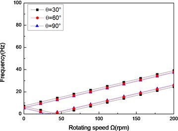
a) First mode

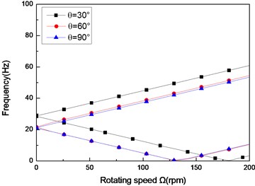
b) Second mode

c) Third mode

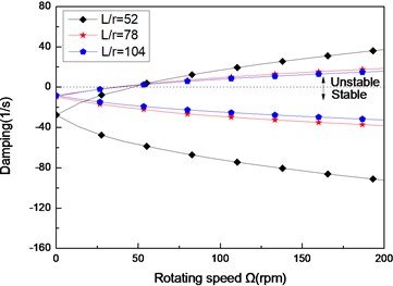
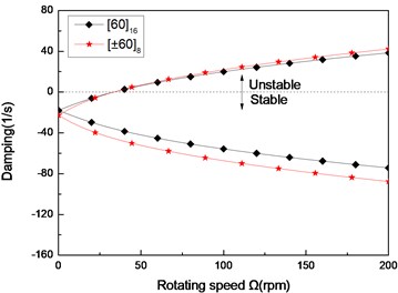
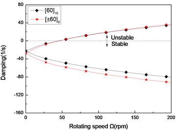
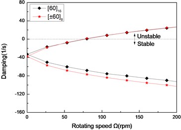
Fig. 3The damping of a simply supported composite shaft versus rotating speed for different ply angles (L/r= 52, θ/-θ8)

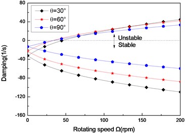
a) First mode

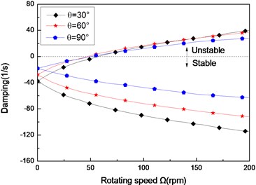
b) Second mode

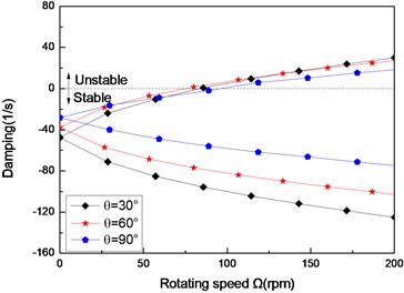
c) Third mode

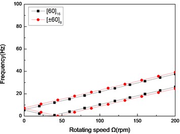
Fig. 4The natural frequency of a simply supported composite shaft versus rotating speed for different length aspect ratios (60/-608)

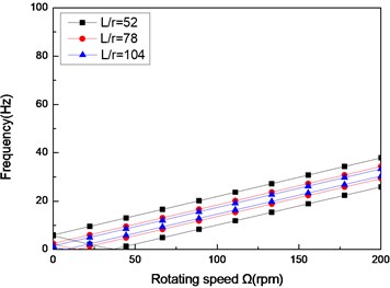
a) First mode

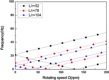
b) Second mode

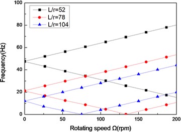
c) Third mode

Figs. 3(a)-(c) present the first three flexural dampings with respect rotating speed for different ply angles. It is evident that as the rotating speed increases, the dampings of the backward modes decrease and are negative, this means the motion involving backward modes is stable. The dampings involving the forward modes are negative at the lower value of $Ω$ and increase with $Ω$ increasing, and at a certain value of $Ω$ the dampings become zero and then are positive. The value of $Ω$ corresponding to zero damping is called as the threshold of instability. Furthermore, it can also be seen that the threshold of instability decreases with ply angle, which is explained by the fact the closer the fiber is oriented to 90°, the higher the internal damping of composite (see specific damping capacity given in Table 3), thus, the lower threshold of instability is. Comparing with the lower mode, the higher modes have larger threshold of instability. This shows that the higher modes are more stable.

Figs. 4 and Figs. 5 show the first three natural frequencies and flexural dampings with respect rotating speed for various length aspect ratios. The results show that as the length aspect ratio increases, the non-rotating natural frequencies decrease and a corresponding decrease in the instability thresholds is also experienced. It can be concluded that for relatively large value of length aspect ratio, the shaft becomes less stability than for low length aspect ratio. A similar conclusion has been arrived by Sino, et al. [14].

As the results reveal, the higher mode is much stronger affected by length aspect ratio, than the lower mode.

Figs. 6 and 7 show the first three natural frequencies and and flexural dampings with respect rotating speed for two typical stacking sequences. The results show that stacking sequence can be used to increase the stability of the rotating composite shaft. From these figures it is evident that the effect of the stacking sequences on the higher modes are significant.

Fig. 5The damping of a simply supported composite shaft versus rotating speed for different length aspect ratios (60/-608)

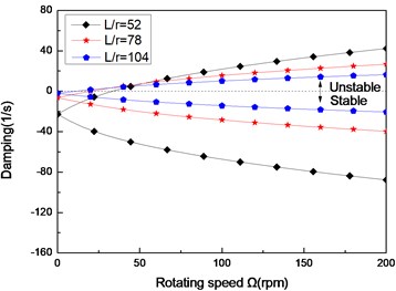
a) First mode

b) Second mode

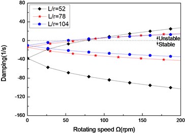
c) Third mode

Fig. 6The natural frequency of a simply supported composite shaft versus rotating speed for different stacking sequences (L/r= 52)

a) First mode

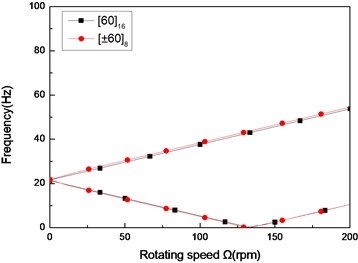
b) Second mode

c) Third mode

Fig. 7The damping of a simply supported composite shaft versus rotating speed for different stacking sequences (L/r= 52)

a) First mode

b) Second mode

c) Third mode

Fig. 8The natural frequency of a composite shaft versus rotating speed for different boundary conditions (L/r= 52, 60/-608)

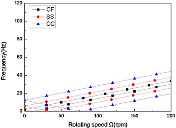
a) First mode

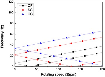
b) Second mode

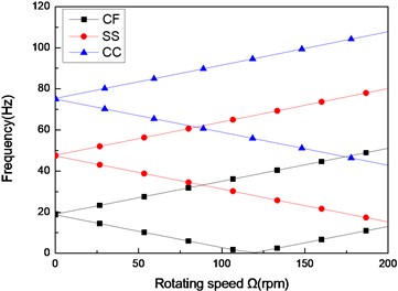
c) Third mode

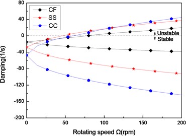
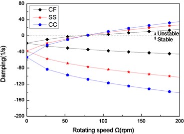
Fig. 9The damping of a composite shaft versus rotating speed for different boundary conditions (L/r= 52, 60/-608)

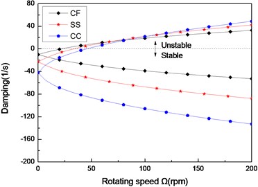
a) First mode

b) Second mode

c) Third mode

Figs. 8 and Figs. 9 show the first three natural frequencies and flexural dampings with respect rotating speed for three different boundary conditions. The results show that boundary condition has a significant effect on the stability of the rotating composite shaft. From Figs. 8, it is obviously that the boundary conditions can exert a great influence over the natural frequency of the higher modes.

Figs. 10 and 11 show the first critical speeds and instability thresholds with respect ply angle for various length aspect ratios, respectively. The results show that the first critical speed and instability threshold decrease with the ply angle and increase with a decrease in length aspect ratio. These trends are consistent with that presented in Figs. 2-5.

Figs. 12 and 13 show the effect of three different boundary conditions on the first critical speeds and instability thresholds of the shaft, respectively. The results show that the maximum critical speed and instability threshold occur for the clamped-clamped (CC) shaft, the minimum ones for the clamped-free (CF) shaft, while the intermediate ones occur for the simply supported (SS) shaft.

Figs. 14 and 15 show the effect of the stacking sequence on the first critical speeds and instability thresholds of the shaft, respectively. The effect of the stacking sequence on the first critical speed and instability threshold is similar to those indicated in Figs. 6 and 7. It can be observed that the angle-ply ${[\pm θ]}_{8}$ seems to exert a larger stabilizing effect, as compared to the stacking sequence ${[θ]}_{16}$ .

Convergence studies with our model indicate that five mode shape functions are sufficient to obtain the accurate results of the first critical speeds and instability thresholds for simply supported shaft as shown in Table 4. This shows that our model is sufficiently accurate even when only a small number of mode shape functions are used.

Fig. 10The variation of critical speeds with ply angle for different length aspect ratios (θ/-θ8, simply supported)

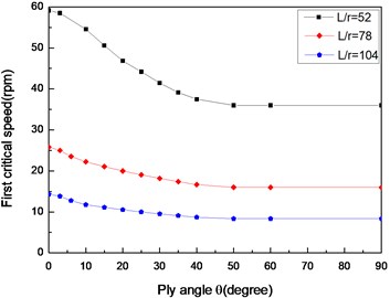
Fig. 11The variation of instability thresholds with ply angle for different length aspect ratios (θ/-θ8, simply supported)

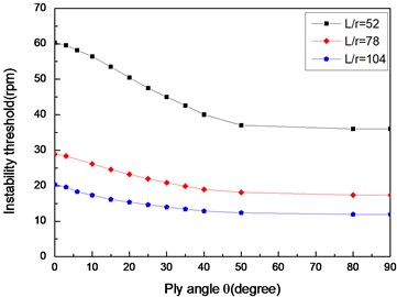
Fig. 12The variation of critical speeds with ply angle for different boundary conditions (L/r= 52, θ/-θ8)

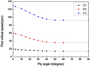
Fig. 13The variation of instability thresholds with ply angle for different boundary conditions (L/r= 52, θ/-θ8)

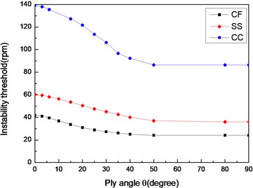
Fig. 14The variation of critical speeds with ply angle for different stacking sequences (L/r= 52, simply supported)

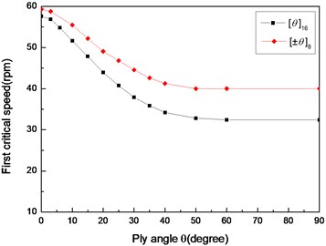
Fig. 15The variation of instability thresholds with ply angle for different stacking sequences (L/r= 52, simply supported)

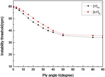
Table 4Effect of model number N on first critical speed and instability threshold (L/r= 52, θ/-θ8 simply supported)

Ply angle (degree)	First critical speed (rpm)			Instability threshold (rpm)
Ply angle (degree)	$N =$ 1	$N =$ 3	$N =$ 5	$N =$ 1	$N =$ 3	$N =$ 5
30	44.65	44.72	44.72	45.47	45.62	45.62
60	40.44	40.64	40.64	42.03	42.35	42.35
90	36.58	36.67	36.67	38.03	38.23	38.23

4. Conclusions

A refined variational asymptotic approach and Galerkin’s method was used to model the free vibration equations and to predict the dynamical behavior the rotating composite Timoshenko shafts with internal damping. The present numerical results are compatible to those available in the literature. The critical speeds and instability thresholds are obtained using the present model. From the presented results, the following conclusions can be made:

1) The proper stacking sequence is useful for increasing critical rotating speeds and instability thresholds of composite shaft.

2) The clamped-clamped composite shaft has the higher critical rotating speed and threshold of instability and consequently better dynamic stability than the shaft with other boundary conditions

3) The ply angles up to 50°have a significant effect on dynamics of composite shaft and at the ply angle 0°, maximum critical speed and instability threshold are reached. However, for the ply angles in the range 50°-90°, their effect appears to be marginal.

4) The instability threshold is always higher than the critical rotating speed.

References

Zinberg H., Symonds M. F. The development of an advanced composite tail rotor drive shaft. Presented at the 26th Annual National Forum of the American Helicopter Society, Washington, DC, 1970.

Search CrossRef
dos Reis H. L. M., Goldman R. B., Verstrate P. H. Thin-walled laminated composite cylindrical tubes; part 3 – critical speed analysis. Journal of Composites Technology and Research, Vol. 9, 1987, p. 58-62.

Search CrossRef
Kim C. D., Bert C. W. Critical speed analysis of laminated composite, hollow drive shafts. Composites Engineering, Vol. 3, 1993, p. 633-643.

Search CrossRef
Singh S. P., Gupta K. Composite shaft rotordynamic analysis using a layerwise theory. Journal of Sound and Vibration, Vol. 191, Issue 5, 1996, p. 739-756.

Search CrossRef
Chang M. Y., Chen J. K., Chang C. Y. A simple spinning laminated composite shaft model. International Journal of Solids and Structures, Vol. 41, 2004, p. 637-662.

Search CrossRef
Gubran H. B. H., Gupta K. The effect of stacking sequence and coupling mechanisms on the natural frequencies of composite shafts. Journal of Sound and Vibration Vol. 282, 2005, p. 231-48.

Search CrossRef
Song O., Jeong N.-H., Librescu L. Implication of conservative and gyroscopic forces on vibration and stability of an elastically tailored rotating shaft modeled as a composite thin-walled beam. Journal of Acoustical Society of America, Vol. 109, Issue 3, 2001, p. 972-981.

Search CrossRef
Rehfield L. W. Design analysis methodology for composite rotor blades. Proceedings of the 7th DoD/NASA Conference on Fibrous Composites in Structural Design, 1985.

Search CrossRef
Ren Yongsheng, Dai Qiyi, Zhang Xingqi Modeling and dynamic analysis of rotating composite shaft. Journal of Vibroengineering, Vol. 15, Issue 4, 2013, p. 1816-1832.

Search CrossRef
Singh S. P., Gupta K. Free damped flexural vibration analysis of composite cylindrical tubes using beam and shell theories. Journal of Sound and Vibration, Vol. 172, Issue 2, 1994, p. 171-90.

Search CrossRef
Kim W., Argento A., Scott R. A. Forced vibration and dynamic stability of a rotating tapered composite Timoshenko shaft: bending motions in end-milling operations. Journal of Sound and Vibration, Vol. 246, 2001, p. 563-600.

Search CrossRef
Mazzei A. J., Scott R. A. Effects of internal viscous damping on the stability of a rotating shaft driven through a universal joint. Journal of Sound and Vibration, Vol. 265, 2003, p. 863-885.

Search CrossRef
Montagnier O., Hochard C. H. Dynamics of a supercritical composite shaft mounted on viscoelastic supports. Journal of Sound and Vibration, Vol. 333, 2014, p. 470-484.

Search CrossRef
Sino R., Baranger T. N., Chatelet E., Jacquet G. Dynamic analysis of a rotating composite shaft. Composites Science and Technology, Vol. 68, 2008, p. 337-345.

Search CrossRef
Ren Yongsheng, Zhang Xingqi, Liuyanghang, Chen Xiulong Vibration and instability of rotating composite thin-walled shafts with internal damping. Shock and Vibration, 2014, p. 123271-1-10.

Search CrossRef
Berdichevsky V. L., Armanios E., Badir A. M. Theory of anisotropic thin-walled closed-cross-section beams. Composites Engineering, Vol. 2, Issues 5-7, 1992, p. 411-432.

Search CrossRef
Ren Yongsheng, Du Xianghong, Sun Shuangshuang, Teng Xiangmeng Structure damping of thin-walled composite one-cell beams. Journal of Vibration and Shock, Vol. 31, Issue 3, 2012, p. 141-152, (in Chinese).

Search CrossRef
Dharmarajan S., Mccutchen H. Shear coefficients for orthotropic beams. Journal of Composite Materials,Vol. 7, 1973, p. 530-535.

Search CrossRef
Smith E. C., Chopra I. Formulation and evaluation of an analytical model for composite box-beams. Journal of American Helicopter Society, Vol. 36, Issue 3, 1991, p. 23-25.

Search CrossRef
Saravanos D. A., Varelis D., Plagianakos T. S., et al. A shear beam finite element for the damping analysis of tubular laminated composite beams. Journal of Sound and Vibration, Vol. 291, 2006, p. 802-823.

Search CrossRef
Banerjee J. R., Su H. Development of a dynamic stiffness matrix for free vibration analysis of spinning beams. Computer and Structures, Vol. 82, 2004, p. 2189-2197.

Search CrossRef

About this article

Received

03 April 2015

Accepted

12 November 2015

Published

30 December 2015

SUBJECTS

Modal analysis

Keywords

composite shaft

internal damping

vibration and stability

Acknowledgements

The research is funded by the National Natural Science Foundation of China (Grant No. 11272190), Shandong Provincial Natural Science Foundation of China (Grant No. ZR2011EEM031).

This is an open access article distributed under the Creative Commons Attribution License, which permits unrestricted use, distribution, and reproduction in any medium, provided the original work is properly cited.