Nonlinear oscillations and chaotic dynamics of a supported FGM rectangular plate system under mixed excitations

Hamed, Yasser S.

Journal of Vibroengineering

Browse Journal

Submit article

Published: 15 November 2014

Check for updates

Nonlinear oscillations and chaotic dynamics of a supported FGM rectangular plate system under mixed excitations

Yasser S. Hamed¹

¹Department of Mathematics and Statistics, Faculty of Science, Taif University, El-Taif, El-Haweiah, P.O. Box 888, Zip Code 21974, Kingdom of Saudi Arabia

¹Department of Engineering Mathematics, Faculty of Electronic Engineering, Menouf, 32952, Egypt

Cite the article Download PDF

Downloads 1159

WoS Core Citations 3

Abstract

In this paper, we investigated the nonlinear oscillations, vibrations and chaotic dynamics of a simply supported rectangular plate made of functionally graded materials (FGMs) through a temperature field subjected to mixed excitations. The rectangular FGM plate system described by a coupled of nonlinear differential equations (two degree of freedom) including the quadratic and cubic nonlinear terms. The mathematical solutions of the governing equations of motion for the FGM plate derived using the perturbation method based on the power series expansion up to and including the second order approximation. The numerical simulations investigated using Runge-Kutta of fourth order using MATLAB and MAPLE programs. All different resonance cases reported and studied numerically. We applied both frequency response equations and phase-plane technique and also Lyapunov’s first method near the worst resonance cases to analyze the stability of the steady state solution of vibrating system. The effects of the different parameters of the rectangular plate system studied numerically. Results compared to previously published work. In the future work, we can deal with the same system subjected multi-external and tuned and parametric excitation forces. Also, the system can be studied at another worst different resonance cases, active and passive controller.

1. Introduction

The functionally graded materials (FGMs) have received a considerable attention recently as one class of inhomogeneous composite materials. Functionally graded materials (FGMs) are inhomogeneous composites within which materials properties vary continuously. This is achieved by gradually changing the composition of the constituent materials, usually in one direction, to obtain smooth variation in material properties [1]. Reddy [2] developed both theoretical and finite element formulations for thick FGM plates according to the higher-order shear deformation plates theory, and studied the non-linear dynamic response of FGM plates subjected to a sudden applied uniform pressure. Yang et al. [3] studied the large amplitude vibration of pre-stressed FGM laminated plates that were composed of an FGM layer and two surface-mounted piezoelectric actuator layers. Huang and Shen [4] dealt with the nonlinear vibration and dynamic response of FGM plates in heat environment. Heat conduction and temperature-dependent material properties were both considered. More recently, Yang and his coworkers studied the sensitivity of nonlinear vibration and dynamic response of FGM plates to initial geometrical imperfections of arbitrary shape [5, 6]. Ye et al. [7] dealt with nonlinear dynamic behavior of a parametrically excited, simply supported, symmetric cross-ply laminated rectangular thin plate. The geometric nonlinearity and nonlinear damping were included in the governing equations of motion. FGM were initially designed as thermal barriers for aerospace structures and fusion reactors. Usually, they are made from a mixture of metals and ceramics. Due to their unique advantage of being able to withstand sever high-temperature, FGM have found a wide range of applications in many industries, especially in space vehicles and aircrafts, where they are often subjected to high levels of thermal and dynamic loading, such as large temperature gradients and acoustic pressure, which may result in a complicated nonlinear vibration behavior of the FGM plate structures [8]. Hao et al. [9] established the nonlinear governing equations of motion for a simply supported FGM rectangular plate subjected to the transversal and in-plane excitations in thermal environment and investigated the nonlinear oscillations, bifurcations and chaos of the functionally graded material plate. Zhang et al. [10] studied the chaotic vibrations of an orthotropic FGM rectangular plate based on third-order shear deformation theory. Zhang et al. [10] investigated the nonlinear vibrations and chaotic dynamics of a simply supported orthotropic FGM rectangular plate subjected to the in-lane and transverse excitations together with thermal loading. The present study is focused on the case of 1:2:4 internal resonance, primary parametric resonance and sub-harmonic resonance of order 1/2. Yang et al. [11] analyzed the nonlinear dynamic responses of a functionally graded plate with a through-width surface crack. Li et al. [12] used the extended Melnikov method to investigate the multi-pulse chaotic dynamics of a functionally graded material rectangular plate with one-to-one internal resonance. Malekzadeh [13] studied free vibration of functionally graded (FG) thin-to-moderately thick annular plates subjected to thermal environment and supported on two-parameter elastic foundation. Akbarzadeh et al. [14] investigated the dynamic response of a simply supported functionally graded rectangular plate subjected to a lateral thermomechanical by using the hybrid Fourier-Laplace transform method. Zhang et al. [15] investigated the nonlinear periodic and chaotic motions of a simply supported FGM rectangular plate under both in plane and transverse excitations in thermal environment. The present analysis is focused on the case of 1:2 internal resonance and primary parametric resonance, 1/2 sub-harmonic resonance. Eissa and Sayed [16-18], studied the effects of different active controllers on simple and spring pendulum at the primary resonance via negative velocity feedback or it’s square or cubic. Hamed et al. [19-21] studied USM model subject to multi-external or both multi-external and multi-parametric and both multi-external and tuned excitation forces. The model consists of multi-degree-of-freedom system consisting of the tool holder and absorbers (tools) simulating ultrasonic machining process. The advantages of using multi-tools are to machine different materials and different shapes at the same time. This leads to time saving and higher machining efficiency. Sayed and Hamed [22] studied the response of a two-degree-of-freedom system with quadratic coupling under parametric and harmonic excitations. The method of multiple scale perturbation technique is applied to solve the non-linear differential equations and obtain approximate solutions up to and including the second-order approximations. Hamed et al [23] presented the behavior of the nonlinear string beam coupled system subjected to external, parametric and tuned excitations for case 1:1 internal resonance. The stability of the system studied using frequency response equations and phase-plane method. It is found from numerical simulations that there are obvious jumping phenomena in the frequency response curves. Sayed and et al. [24] investigated the non-linear dynamics of a two-degree-of freedom vibration system including quadratic and cubic non-linearities subjected to external and parametric excitation forces. There exist multi-valued solutions which increase or decrease by the variation of some parameters. The numerical simulations show the system exhibits periodic motions and chaotic motions. Amer and Sayed [25] studied the response of one-degree-of freedom, non-linear system under multi-parametric and external excitation forces simulating the vibration of the cantilever beam. The solution of this system up to and including the second order approximation is determined applying the multiple time scale perturbation. The steady state solution and its stability are determined. Sayed and Kamel [26, 27] investigated the effect of different controllers on the vibrating system and the saturation control of a linear absorber to reduce vibrations due to rotor blade flapping motion. The stability of the obtained numerical solution is investigated using both phase plane methods and frequency response equations. Sayed and Mousa [28] investigated the influence of the quadratic and cubic terms on non-linear dynamic characteristics of the angle-ply composite laminated rectangular plate with parametric and external excitations. They focused on the case of 1:2 internal resonance and sub-harmomic resonance. Sayed and Mousa [29] investigated the perturbation method and stability of the composite laminated piezoelectric rectangular plate under simultaneous transverse and in-plane excitations. They focused on the case of 1:1:3 internal resonance and primary resonance. The stability of the system and the effects of different parameters on system behavior have been studied using frequency response curves. Stability is performed of figures by solid and dotted lines. The analytical results given by the method of multiple time scale is verified by comparison with results from numerical integration of the modal equations. It is quite clear that some of the simultaneous resonance cases are undesirable in the design of such system.

2. Mathematical analysis

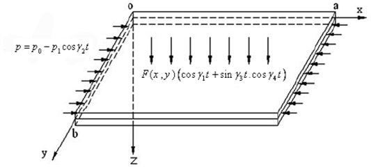
A simply supported FGM rectangular plate subjected to a through-thickness temperature field together with tuned, parametric and external excitations is considered in this study. The plate is of length $a$ , width $b$ , and thickness $h$ as shown in Fig. 1. Assume that ( $u, v, w$ ) represent the displacements of an arbitrary point of the FGM rectangular plate in the $x$ , $y$ , and $z$ directions respectively. Along the plate edges $x =$ 0, $x = a$ , the plate is subjected to an in-plane excitation $p = p_{0} - p_{1} c o s γ_{2} t$ where $p_{0}$ , $p_{1}$ are the external excitation amplitude in $y$ direction and a transverse excitation $F (x, y) (c o s γ_{1} t + s i n γ_{3} t * c o s γ_{4} t)$ , where $F (x, y)$ are the parametric and tuned excitation amplitudes in $z$ direction. Here $ϕ_{x}$ and $ϕ_{y}$ represent the mid-plane rotations of a transverse normal about the $y$ and $x$ axes, $γ_{1}$ , $γ_{2}$ , $γ_{3}$ and $γ_{4}$ are the excitation frequencies of the transverse and in-plane excitations, respectively. According to the Reddy’s third-order shear deformation plate theory (TSDT) [30], the displacement field of the plate is assumed as:

1a

u (x, y, t) = u_{0} (x, y, t) + z ϕ_{x} (x, y, t) - c_{1} z^{3} (ϕ_{x} + \frac{\partial w_{0}}{\partial x}),

1b

v (x, y, t) = v_{0} (x, y, t) + z ϕ_{y} (x, y, t) - c_{1} z^{3} (ϕ_{y} + \frac{\partial w_{0}}{\partial y}),

1c

w (x, y, t) = w_{0} (x, y, t),

where ( $u_{0}, v_{0}, w_{0}$ ) represent the displacements of a point in middle plane of the FGM rectangular plate in the $x$ , $y$ , and $z$ directions respectively. According to the von Karman strain-displacements relationship and the Hamilton’s principle, the nonlinear governing equations of motion for the FGM rectangular plate are derived as:

2a

N_{x x, x} + N_{x y, y} = I_{0} {\ddot{u}}_{0} + (I_{1} - c_{1} I_{3}) {\ddot{ϕ}}_{x} - c_{1} I_{3} \frac{\partial {\ddot{w}}_{0}}{\partial x},

2b

N_{y y, y} + N_{x y, y} = I_{0} {\ddot{v}}_{0} + (I_{1} - c_{1} I_{3}) {\ddot{ϕ}}_{y} - c_{1} I_{3} \frac{\partial {\ddot{w}}_{0}}{\partial y},

2c

N_{y y, y} \frac{\partial w_{0}}{\partial y} + N_{y y} \frac{\partial^{2} w_{0}}{\partial y^{2}} + N_{x y, y} \frac{\partial w_{0}}{\partial x} + N_{x y, x} \frac{\partial w_{0}}{\partial y} + 2 N_{x y} \frac{\partial^{2} w_{0}}{\partial y \partial x} + N_{x x, x} \frac{\partial w_{0}}{\partial x} + N_{x x} \frac{\partial^{2} w_{0}}{\partial x^{2}}

+ c_{1} (p_{x x, x x} + 2 p_{x y, x y} + p_{y y, y y}) + (Q_{x, x} - c_{2} R_{x, x}) + (Q_{y, y} - c_{2} R_{y, y}) + F - γ {\dot{w}}_{0}

= I_{0} {\ddot{w}}_{0} + c_{1} I_{3} (\frac{\partial {\ddot{u}}_{0}}{\partial x} + \frac{\partial {\ddot{v}}_{0}}{\partial y}) + (c_{1} I_{4} - c_{1}^{2} I_{6}) (\frac{\partial {\ddot{ϕ}}_{x}}{\partial x} + \frac{\partial {\ddot{ϕ}}_{y}}{\partial y}) - c_{1}^{2} I_{6} (\frac{\partial^{2} {\ddot{w}}_{0}}{\partial x^{2}} + \frac{\partial^{2} {\ddot{w}}_{0}}{\partial y^{2}}),

2d

M_{x x, x} + M_{x y, y} - c_{1} (p_{x x, x} + p_{x y, y}) - (Q_{x} - c_{2} R_{x}) = (I_{1} - c_{1} I_{3}) {\ddot{u}}_{0}

+ (I_{2} - 2 c_{1} I_{4} + c_{1}^{2} I_{6}) {\ddot{ϕ}}_{x} - (c_{1} I_{4} - c_{1}^{2} I_{6}) \frac{\partial {\ddot{w}}_{0}}{\partial x},

2e

M_{y y, y} + M_{x y, y} - c_{1} (p_{y y, y} + p_{x y, x}) - (Q_{y} - c_{2} R_{y}) = (I_{1} - c_{1} I_{3}) {\ddot{v}}_{0}

+ (I_{2} - 2 c_{1} I_{4} + c_{1}^{2} I_{6}) {\ddot{ϕ}}_{y} - (c_{1} I_{4} - c_{1}^{2} I_{6}) \frac{\partial {\ddot{w}}_{0}}{\partial y} .

The boundary conditions for the simply supported plate under current consideration require at:

3a

x = 0, x = a, w = ϕ_{y} = M_{x x} = p_{x x} = N_{x y} = 0,

3b

y = 0, y = b, w = ϕ_{x} = M_{y y} = p_{y y} = N_{x y} = 0,

3c

N_{y y} |_{y = 0, b} = 0, \int_{0}^{b} N_{x x} |_{x = 0, a} d y = - \int_{0}^{b} (p_{0} - p_{1} c o s γ_{2} t) d y .

Fig. 1The model of a rectangular FGM plate and the coordinate system

Applying the Galerkin procedure yield the dimensionless governing differential equation of transverse motion of the FGM rectangular plate with two degrees of freedom as follows:

The governing differential equation of transverse motion of the FGM rectangular plate with two degrees of freedom as follows:

4a

\ddot{x} + ω_{1}^{2} x = ε (- β_{1} x^{2} - β_{2} y^{2} - β_{3} x^{3} - β_{4} x y^{2} - β_{5} x y)

+ ε^{2} (ρ_{1} c o s γ_{1} t - ρ_{11} x c o s γ_{2} t + ρ_{21} s i n γ_{3} t * c o s γ_{4} t - μ_{1} \dot{x}),

4b

\ddot{y} + ω_{2}^{2} y = ε (- η_{1} y^{2} - η_{2} x^{2} - η_{3} y^{3} - η_{4} x^{2} y - η_{5} x y)

+ ε^{2} (ρ_{2} c o s γ_{1} t - ρ_{12} y c o s γ_{2} t + ρ_{22} s i n γ_{3} t * c o s γ_{4} t - μ_{2} \dot{y}) .

The initial conditions for the simply supported plate are:

5

x (t = 0) = 0, y (t = 0) = 0, \dot{x} (t = 0) = 0, \dot{y} (t = 0) = 0,

where $x$ and $y$ are the amplitudes of the FGM rectangular plate for the first and second modes, $ω_{1}$ and $ω_{2}$ the natural frequencies of the rectangular plate modes, $μ_{1}$ and $μ_{2}$ are the modal damping coefficients, and $γ_{1}$ , $γ_{2}$ , $γ_{3}$ and $γ_{4}$ are the external and parametric and tuned excitation frequencies respectively. $ρ_{1}$ , $ρ_{2}$ , $ρ_{11}$ , $ρ_{12}$ , $ρ_{21}$ and $ρ_{22}$ are related to the magnitude of the excitation forces of the FGM rectangular plate modes, $ε$ is a small perturbation parameter and $0 < ε < < 1$ . We introducing three time scales:

6

T_{0} = t, T_{1} = ε t, T_{2} = ε^{2} t .

We seek an asymptotic solution of Eq. (4) for $x$ and $y$ in the form:

7a

x (t, ε) = x_{10} (T_{0}, T_{1}, T_{2}) + ε x_{11} (T_{0}, T_{1}, T_{2}) + ε^{2} x_{12} (T_{0}, T_{1}, T_{2}) + O (ε^{3}),

7b

y (t, ε) = y_{10} (T_{0}, T_{1}, T_{2}) + ε y_{11} (T_{0}, T_{1}, T_{2}) + ε^{2} y_{12} (T_{0}, T_{1}, T_{2}) + O (ε^{3}) .

Derivatives with respect to $t$ are then transformed into:

8a

\frac{d}{d t} = D_{0} + ε D_{1} + ε^{2} D_{2},

8b

\frac{d^{2}}{d t^{2}} = D_{0}^{2} + 2 ε D_{0} D_{1} + ε^{2} (D_{1}^{2} + 2 D_{0} D_{2}) .

The derivatives $\dot{x}$ , $\dot{y}$ , $\ddot{x}$ and $\ddot{y}$ are in the form:

9a

\dot{x} = D_{0} x_{10} + ε (D_{0} x_{11} + D_{1} x_{10}) + ε^{2} (D_{0} x_{12} + D_{1} x_{11} + D_{2} x_{10}),

9b

\ddot{x} = D_{0}^{2} x_{10} + ε (D_{0}^{2} x_{11} + 2 D_{0} D_{1} x_{10}) + ε^{2} (D_{0}^{2} x_{12} + 2 D_{0} D_{1} x_{11} + D_{1}^{2} x_{10} + 2 D_{0} D_{2} x_{10}),

9c

\dot{y} = D_{0} y_{10} + ε (D_{0} y_{11} + D_{1} y_{10}) + ε^{2} (D_{0} y_{12} + D_{1} y_{11} + D_{2} y_{10}),

9d

\ddot{y} = D_{0}^{2} y_{10} + ε (D_{0}^{2} y_{11} + 2 D_{0} D_{1} y_{10}) + ε^{2} (D_{0}^{2} y_{12} + 2 D_{0} D_{1} y_{11} + D_{1}^{2} y_{10} + 2 D_{0} D_{2} y_{10}),

where $D_{n} = \partial / \partial T_{n}$ , $n =$ 0, 1, 2. Terms of $O (ε^{3})$ and higher orders are neglected. Substituting Eqs. (7)-(9) into Eq. (4) we get:

10a

(D_{0}^{2} x_{10} + ε (D_{0}^{2} x_{11} + 2 D_{0} D_{1} x_{10}) + ε^{2} (D_{0}^{2} x_{12} + 2 D_{0} D_{1} x_{11} + D_{1}^{2} x_{10} + 2 D_{0} D_{2} x_{10}))

+ ω_{1}^{2} (x_{10} + ε x_{11} + ε^{2} x_{12})

= ε (\begin{matrix} - β_{1} {(x_{10} + ε x_{11} + ε^{2} x_{12})}^{2} - β_{2} {(y_{10} + ε y_{11} + ε^{2} y_{12})}^{2} \\ - β_{3} {(x_{10} + ε x_{11} + ε^{2} x_{12})}^{3} - β_{4} (x_{10} + ε x_{11} + ε^{2} x_{12}) {(y_{10} + ε y_{11} + ε^{2} y_{12})}^{2} \\ - β_{5} (x_{10} + ε x_{11} + ε^{2} x_{12}) (y_{10} + ε y_{11} + ε^{2} y_{12}) \end{matrix})

+ ε^{2} (\begin{matrix} ρ_{1} c o s γ_{1} t - ρ_{11} (x_{10} + ε x_{11} + ε^{2} x_{12}) c o s γ_{2} t + ρ_{21} s i n γ_{3} t c o s γ_{4} t \\ - μ_{1} (D_{0} x_{10} + ε (D_{0} x_{11} + D_{1} x_{10}) + ε^{2} (D_{0} x_{12} + D_{1} x_{11} + D_{2} x_{10})) \end{matrix}),

10b

(D_{0}^{2} y_{10} + ε (D_{0}^{2} y_{11} + 2 D_{0} D_{1} y_{10}) + ε^{2} (D_{0}^{2} y_{12} + 2 D_{0} D_{1} y_{11} + D_{1}^{2} y_{10} + 2 D_{0} D_{2} y_{10}))

+ ω_{2}^{2} (y_{10} + ε y_{11} + ε^{2} y_{12})

= ε (\begin{matrix} - η_{1} {(y_{10} + ε y_{11} + ε^{2} y_{12})}^{2} - η_{2} {(x_{10} + ε x_{11} + ε^{2} x_{12})}^{2} \\ - η_{3} {(y_{10} + ε y_{11} + ε^{2} y_{12})}^{3} - η_{4} {(x_{10} + ε x_{11} + ε^{2} x_{12})}^{2} (y_{10} + ε y_{11} + ε^{2} y_{12}) \\ - η_{5} (x_{10} + ε x_{11} + ε^{2} x_{12}) (y_{10} + ε y_{11} + ε^{2} y_{12}) \end{matrix})

+ ε^{2} (\begin{matrix} ρ_{2} c o s γ_{1} t - ρ_{12} (y_{10} + ε y_{11} + ε^{2} y_{12}) c o s γ_{2} t + ρ_{22} s i n γ_{3} t c o s γ_{4} t \\ - μ_{2} (D_{0} y_{10} + ε (D_{0} y_{11} + D_{1} y_{10}) + ε^{2} (D_{0} y_{12} + D_{1} y_{11} + D_{2} y_{10})) \end{matrix}) .

We expand the two sides of Eqs. (10) and equating the coefficients of similar powers of $ε$ , one obtains the following set of ordinary differential equations:

Order $ε^{0}$ :

11a

(D_{0}^{2} + ω_{1}^{2}) x_{10} = 0,

11b

(D_{0}^{2} + ω_{2}^{2}) y_{10} = 0 .

Order $ε^{1}$ :

12a

(D_{0}^{2} + ω_{1}^{2}) x_{11} = - 2 D_{0} D_{1} x_{10} - β_{1} x_{10}^{2} - β_{2} y_{10}^{2} - β_{3} x_{10}^{3} - β_{4} x_{10} y_{10}^{2} - β_{5} x_{10} y_{10},

12b

(D_{0}^{2} + ω_{2}^{2}) y_{11} = - 2 D_{0} D_{1} y_{10} - η_{1} y_{10}^{2} - η_{2} x_{10}^{2} - η_{3} y_{10}^{3} - η_{4} y_{10} x_{10}^{2} - η_{5} y_{10} x_{10} .

Order $ε^{2}$ :

13a

(D_{0}^{2} + ω_{1}^{2}) x_{12} = - 2 D_{0} D_{2} x_{10} - D_{1}^{2} x_{10} - 2 D_{0} D_{1} x_{11} - 2 β_{1} x_{10} x_{11} - 2 β_{2} y_{10} y_{11}

- 3 β_{3} x_{10}^{2} x_{11} - μ_{1} D_{0} x_{10} - β_{4} (x_{11} y_{10}^{2} + 2 x_{10} y_{10} y_{11}) - β_{5} (x_{10} y_{11} + x_{11} y_{10})

- ρ_{11} x_{10} c o s γ_{2} t + ρ_{1} c o s γ_{1} t + ρ_{21} s i n γ_{3} t c o s γ_{4} t,

13b

(D_{0}^{2} + ω_{2}^{2}) y_{12} = - 2 D_{0} D_{2} y_{10} - D_{1}^{2} y_{10} - 2 D_{0} D_{1} y_{11} - 2 η_{1} y_{10} y_{11} - 2 η_{2} x_{10} x_{11}

- 3 η_{3} y_{10}^{2} y_{11} - μ_{2} D_{0} y_{10} - η_{4} (y_{11} x_{10}^{2} + 2 y_{10} x_{10} x_{11}) - η_{5} (y_{10} x_{11} + y_{11} x_{10})

- ρ_{12} y_{10} c o s γ_{2} t + ρ_{2} c o s γ_{1} t + ρ_{22} s i n γ_{3} t c o s γ_{4} t .

The general solutions of Eq. (11), can be written in the form:

14a

x_{10} = A_{1} e x p (i ω_{1} T_{0}) + {\bar{A}}_{1} e x p (- i ω_{1} T_{0}),

14b

y_{10} = A_{2} e x p (i ω_{2} T_{0}) + {\bar{A}}_{2} e x p (- i ω_{2} T_{0}),

where $A_{1}$ and $A_{2}$ are a complex function in $T_{1}$ , $T_{2}$ . Substituting Eq. (14) into Eq. (12) we get:

15a

(D_{0}^{2} + ω_{1}^{2}) x_{11} = (- 2 D_{0} D_{1} A_{1} - 2 β_{4} A_{1} A_{2} {\bar{A}}_{2} - 3 β_{3} A_{1}^{2} {\bar{A}}_{1}) \exp (i ω_{1} T_{0})

+ (- 2 D_{0} D_{1} {\bar{A}}_{1} - 2 β_{4} {\bar{A}}_{1} {\bar{A}}_{2} A_{2} - 3 β_{3} {\bar{A}}_{1}^{2} A_{1}) \exp (- i ω_{1} T_{0}) - β_{1} A_{1}^{2} \exp (2 i ω_{1} T_{0})

- β_{1} {\bar{A}}_{1}^{2} \exp (- 2 i ω_{1} T_{0}) - β_{2} A_{2}^{2} \exp (2 i ω_{2} T_{0}) - β_{2} {\bar{A}}_{2}^{2} \exp (- 2 i ω_{2} T_{0})

- β_{3} A_{1}^{3} e x p (3 i ω_{1} T_{0}) - β_{3} {\bar{A}}_{1}^{3} e x p (- 3 i ω_{1} T_{0}) - β_{5} A_{1} A_{2} e x p (i (ω_{1} + ω_{2}) T_{0})

- β_{5} {\bar{A}}_{1} {\bar{A}}_{2} \exp (- i (ω_{1} + ω_{2}) T_{0}) - β_{5} A_{1} {\bar{A}}_{2} \exp (i (ω_{1} - ω_{2}) T_{0})

- β_{5} {\bar{A}}_{1} A_{2} \exp (- i (ω_{1} - ω_{2}) T_{0}) - β_{4} A_{1} A_{2}^{2} \exp (i (ω_{1} + 2 ω_{2}) T_{0})

- β_{4} {\bar{A}}_{1} {\bar{A}}_{2}^{2} \exp (- i (ω_{1} + 2 ω_{2}) T_{0}) - β_{4} A_{1} {\bar{A}}_{2}^{2} \exp (i (ω_{1} - 2 ω_{2}) T_{0})

- β_{4} {\bar{A}}_{1} A_{2}^{2} e x p (- i (ω_{1} - 2 ω_{2}) T_{0}) - 2 β_{1} A_{1} {\bar{A}}_{1} - 2 β_{2} A_{2} {\bar{A}}_{2},

15b

(D_{0}^{2} + ω_{2}^{2}) y_{11} = (- 2 D_{0} D_{1} A_{2} - 2 η_{4} A_{1} {\bar{A}}_{1} A_{2} - 3 η_{3} A_{2}^{2} {\bar{A}}_{2}) e x p (i ω_{2} T_{0})

+ (- 2 D_{0} D_{1} {\bar{A}}_{2} - 2 η_{4} {\bar{A}}_{1} A_{1} {\bar{A}}_{2} - 3 η_{3} A_{2} {\bar{A}}_{2}^{2}) e x p (- i ω_{2} T_{0}) - η_{2} A_{1}^{2} e x p (2 i ω_{1} T_{0})

- η_{1} {\bar{A}}_{1}^{2} e x p (- 2 i ω_{1} T_{0}) - η_{1} A_{2}^{2} e x p (2 i ω_{2} T_{0}) - η_{1} {\bar{A}}_{2}^{2} e x p (- 2 i ω_{2} T_{0})

- η_{3} A_{2}^{3} e x p (3 i ω_{2} T_{0}) - η_{3} {\bar{A}}_{2}^{3} e x p (- 3 i ω_{2} T_{0}) - η_{5} A_{1} A_{2} e x p (i (ω_{2} + ω_{1}) T_{0})

- η_{5} {\bar{A}}_{1} {\bar{A}}_{2} e x p (- i (ω_{2} + ω_{1}) T_{0}) - η_{5} A_{2} {\bar{A}}_{1} e x p (i (ω_{2} - ω_{1}) T_{0})

- η_{5} {\bar{A}}_{2} A_{1} e x p (- i (ω_{2} - ω_{1}) T_{0}) - η_{4} A_{2} A_{1}^{2} e x p (i (ω_{2} + 2 ω_{1}) T_{0})

- η_{4} {\bar{A}}_{2} {\bar{A}}_{1}^{2} e x p (- i (ω_{2} + 2 ω_{1}) T_{0}) - η_{4} A_{2} {\bar{A}}_{1}^{2} e x p (i (ω_{2} - 2 ω_{1}) T_{0})

- η_{4} {\bar{A}}_{2} A_{1}^{2} e x p (- i (ω_{2} - 2 ω_{1}) T_{0}) - 2 η_{1} A_{2} {\bar{A}}_{2} - 2 η_{2} A_{1} {\bar{A}}_{1} .

Eliminating the secular terms $e^{(\pm i ω_{1} T_{0})}$ and $e^{(\pm i ω_{2} T_{0})}$ from Eqs. (15), then the first-order approximations are given by:

16a

x_{11} = K_{1} e x p (2 i ω_{1} T_{0}) + K_{2} e x p (2 i ω_{2} T_{0}) + K_{3} e x p (3 i ω_{1} T_{0}) + K_{4} e x p [(i (ω_{1} + ω_{2}) T_{0})]

+ K_{5} e x p [(i (ω_{1} - ω_{2}) T_{0})] + K_{6} e x p [(i (ω_{1} + 2 ω_{2}) T_{0})] + K_{7} e x p [(i (ω_{1} - 2 ω_{2}) T_{0})]

+ K_{8} + c c,

16b

y_{11} = G_{1} e x p (2 i ω_{1} T_{0}) + G_{2} e x p (2 i ω_{2} T_{0}) + G_{3} e x p (3 i ω_{2} T_{0}) + G_{4} e x p [(i (ω_{2} + ω_{1}) T_{0})]

+ G_{5} e x p [(i (ω_{2} - ω_{1}) T_{0})] + G_{6} e x p [(i (ω_{2} + 2 ω_{1}) T_{0})] + G_{7} e x p [(i (ω_{2} - 2 ω_{1}) T_{0})]

+ G_{8} + c c,

where $K_{i}$ , ( $i =$ 1,..., 8) and $G_{i}$ , ( $i =$ 1,..., 8) are a complex function in $T_{1}$ , $T_{2}$ which are given in the appendix and $c c$ stands for the complex conjugate of the preceding terms.

With the same steps used to get the first-order approximation, substituting Eqs. (14), (16) into Eq. (13) and eliminating the secular terms, then the second-order approximations are given by:

17a

x_{12} (T_{0}, T_{1}, T_{2}) = E_{1} e x p (ω_{2} T_{0}) + E_{2} e x p (2 i ω_{1} T_{0}) + E_{3} e x p (2 i ω_{2} T_{0})

+ E_{4} e x p (3 i ω_{1} T_{0}) + E_{5} e x p (3 i ω_{2} T_{0}) + E_{6} e x p (4 i ω_{1} T_{0}) + E_{7} e x p (4 i ω_{2} T_{0})

+ E_{8} e x p (5 i ω_{1} T_{0}) + E_{9} e x p (i (ω_{1} + ω_{2}) T_{0}) + E_{10} e x p (i (ω_{1} - ω_{2}) T_{0})

+ E_{11} e x p (i (ω_{1} + 2 ω_{2}) T_{0}) + E_{12} e x p (i (ω_{1} - 2 ω_{2}) T_{0}) + E_{13} e x p (i (ω_{1} + 3 ω_{2}) T_{0})

+ E_{14} e x p (i (ω_{1} - 3 ω_{2}) T_{0}) + E_{15} e x p (i (ω_{1} + 4 ω_{2}) T_{0}) + E_{16} e x p (i (ω_{1} - 4 ω_{2}) T_{0})

+ E_{17} e x p (i (2 ω_{1} + ω_{2}) T_{0}) + E_{18} e x p (i (2 ω_{1} - ω_{2}) T_{0}) + E_{19} e x p (i (2 ω_{1} + 2 ω_{2}) T_{0})

+ E_{20} e x p (i (2 ω_{1} - 2 ω_{2}) T_{0}) + E_{21} e x p (i (3 ω_{1} + ω_{2}) T_{0}) + E_{22} e x p (i (3 ω_{1} - ω_{2}) T_{0})

+ E_{23} e x p (i (3 ω_{1} + 2 ω_{2}) T_{0}) + E_{24} e x p (i (3 ω_{1} - 2 ω_{2}) T_{0}) + E_{25} e x p (i (γ_{2} + ω_{1}) T_{0})

+ E_{26} e x p (i (γ_{2} - ω_{1}) T_{0}) + E_{27} e x p (i γ_{1} T_{0}) + E_{28} e x p (i (γ_{3} + γ_{4}) T_{0})

+ E_{29} e x p (i (γ_{3} - γ_{4}) T_{0}) + E_{30} + c c,

17b

y_{12} (T_{0}, T_{1}, T_{2}) = H_{1} e x p (ω_{1} T_{0}) + H_{2} e x p (2 i ω_{1} T_{0}) + H_{3} e x p (2 i ω_{2} T_{0})

+ H_{4} e x p (3 i ω_{1} T_{0}) + H_{5} e x p (3 i ω_{2} T_{0}) + H_{6} e x p (4 i ω_{1} T_{0}) + H_{7} e x p (4 i ω_{2} T_{0})

+ H_{8} e x p (5 i ω_{2} T_{0}) + H_{9} e x p (i (ω_{1} + ω_{2}) T_{0}) + H_{10} e x p (i (ω_{1} - ω_{2}) T_{0})

+ H_{11} e x p (i (ω_{1} + 2 ω_{2}) T_{0}) + H_{12} e x p (i (ω_{1} - 2 ω_{2}) T_{0}) + H_{13} e x p (i (ω_{1} + 3 ω_{2}) T_{0})

+ H_{14} e x p (i (ω_{1} - 3 ω_{2}) T_{0}) + H_{15} e x p (i (4 ω_{1} + ω_{2}) T_{0}) + H_{16} e x p (i (4 ω_{1} - ω_{2}) T_{0})

+ H_{17} e x p (i (2 ω_{1} + ω_{2}) T_{0}) + H_{18} e x p (i (2 ω_{1} - ω_{2}) T_{0}) + H_{19} e x p (i (2 ω_{1} + 2 ω_{2}) T_{0})

+ H_{20} e x p (i (2 ω_{1} - 2 ω_{2}) T_{0}) + H_{21} e x p (i (3 ω_{1} + ω_{2}) T_{0}) + H_{22} e x p (i (3 ω_{1} - ω_{2}) T_{0})

+ H_{23} e x p (i (2 ω_{1} + 3 ω_{2}) T_{0}) + H_{24} e x p (i (2 ω_{1} - 3 ω_{2}) T_{0}) + H_{25} e x p (i (γ_{2} + ω_{2}) T_{0})

+ H_{26} e x p (i (γ_{2} - ω_{2}) T_{0}) + H_{27} e x p (i γ_{1} T_{0}) + H_{28} e x p (i (γ_{3} + γ_{4}) T_{0})

+ H_{29} e x p (i (γ_{3} - γ_{4}) T_{0}) + H_{30} + c c,

where $E_{j}$ , ( $j =$ 1,..., 30) and $H_{j}$ , ( $j =$ 1,..., 30) are complex functions in $T_{1}$ , $T_{2}$ and $c c$ represents the complex conjugates.

From the above-derived solutions, many resonance cases can be deduced. The reported resonance cases are classified into:

a) Primary resonance: $γ_{1} ≅ ω_{1}$ , $γ_{1} ≅ ω_{2}$ .

b) Sub-Harmonic resonance: $γ_{2} ≅ 2 ω_{1}$ , $γ_{2} ≅ 2 ω_{2}$ .

c) Internal or secondary resonance: $ω_{2} ≅ ω_{1},$ $ω_{2} ≅ 2 ω_{1},$ $ω_{2} ≅ 3 ω_{1},$ $ω_{2} ≅ 4 ω_{1},$ $ω_{2} ≅ 1 / 2 ω_{1}$ , $ω_{2} ≅ 1 / 3 ω_{1}$ , $ω_{2} ≅ 1 / 4 ω_{1}$ and $ω_{2} ≅ 2 / 3 ω_{1}$ , $ω_{2} ≅ 3 / 2 ω_{1}$ .

d) Combined resonance: $\pm γ_{3} \pm γ_{4} ≅ \pm ω_{1}$ , $\pm γ_{3} \pm γ_{4} ≅ \pm ω_{2}$ .

e) Simultaneous or incident resonance: Any combination of the above resonance cases is considered as simultaneous or incident resonance.

3. Stability of motion

Here, to investigate the stability the simultaneous primary $γ_{1} ≅ ω_{1}$ , combined $γ_{3} - γ_{4} ≅ ω_{1}$ and internal resonance $ω_{2} ≅ 1 / 2 ω_{1}$ are considered. We introduce detuning parameters $σ_{1}$ , $σ_{2}$ and $σ_{3}$ such that:

18

γ_{1} = ω_{1} + ε σ_{1}, γ_{3} - γ_{4} = ω_{1} + ε σ_{2}, 2 ω_{2} = ω_{1} + ε σ_{3} .

This case represents the system worst case. Substituting Eq. (18) into Eqs. (12) and Eq. (13) and eliminating the secular terms, leads to the solvability conditions for the first and second order approximation, we get:

19a

2 i ω_{1} \frac{d A_{1}}{d t} = ε (- 2 β_{4} ω_{1} A_{1} A_{2} {\bar{A}}_{2} - 3 β_{3} A_{1}^{2} {\bar{A}}_{1} - β_{2} A_{2}^{2} \exp (i σ_{3} T_{1}))

+ ε^{2} (- D_{1}^{2} A_{1} - i ω_{1} μ_{1} A_{1} + Γ_{1} A_{1}^{3} {\bar{A}}_{1}^{2} + Γ_{2} A_{1}^{2} {\bar{A}}_{1} A_{2} {\bar{A}}_{2} + Γ_{3} A_{1}^{2} {\bar{A}}_{1} + Γ_{4} A_{1} A_{2}^{2} {\bar{A}}_{2}^{2}

+ Γ_{5} A_{1} A_{2} {\bar{A}}_{2} + (Γ_{6} A_{1} {\bar{A}}_{1} A_{2}^{2} + Γ_{7} A_{2}^{3} {\bar{A}}_{2}) \exp (i σ_{3} T_{1}) + (Γ_{8} A_{1}^{2} {\bar{A}}_{2}^{2}) \exp (- i σ_{3} T_{1})

+ (Γ_{9} {\bar{A}}_{1} A_{2}^{4}) e x p (2 i σ_{3} T_{1}) + \frac{ρ_{1}}{2} e x p (i σ_{1} T_{1}) - \frac{i ρ_{21}}{4} e x p (i σ_{2} T_{1})),

19b

2 i ω_{2} \frac{d A_{2}}{d t} = ε (- 2 η_{4} A_{2} A_{1} {\bar{A}}_{1} - 3 η_{3} A_{2}^{2} {\bar{A}}_{2} - η_{5} {\bar{A}}_{2} A_{1} \exp (- i σ_{3} T_{1}))

+ ε^{2} (- D_{1}^{2} A_{2} - i ω_{2} μ_{2} A_{2} + Γ_{10} A_{2}^{3} {\bar{A}}_{2}^{2} + Γ_{11} A_{2}^{2} {\bar{A}}_{2} A_{1} {\bar{A}}_{1} + Γ_{11} A_{2}^{2} {\bar{A}}_{2} + Γ_{12} A_{2} A_{1}^{2} {\bar{A}}_{1}^{2}

+ Γ_{13} A_{2} A_{1} {\bar{A}}_{1} + (Γ_{14} {\bar{A}}_{1} A_{2}^{3}) e x p (i σ_{3} T_{1}) + (Γ_{15} A_{1}^{2} {\bar{A}}_{2}^{3}) e x p (- 2 i σ_{3} T_{1}) + (Γ_{16} A_{1} A_{2} {\bar{A}}_{2}^{2}

+ Γ_{17} A_{1}^{2} {\bar{A}}_{1} {\bar{A}}_{2}) e x p (- i σ_{3} T_{1})),

where $Γ_{m}$ , ( $m =$ 1,..., 17) are constants.

To analyze the solutions of Eqs. (19), we express $A_{1} (T_{1}, T_{2})$ and $A_{2} (T_{1}, T_{2})$ in the polar form:

20

A_{1} (T_{1}, T_{2}) = \frac{a_{1}}{2} e^{i φ_{1}}, A_{2} (T_{1}, T_{2}) = \frac{a_{2}}{2} e^{i φ_{2}},

where $a_{1}$ , $a_{2}$ and $φ_{1}$ , $φ_{2}$ are the steady state amplitudes and phases of the motion. Substituting Eqs. (20) into Eq. (19) and equating the real and imaginary parts we obtain the following equations describing the modulation of the amplitudes and phases of the first and second modes of FGM rectangular plate response:

21a

{\dot{a}}_{1} = - \frac{μ_{1}}{2} a_{1} + \frac{ρ_{1}}{2 ω_{1}} s i n θ_{1} - \frac{ρ_{21}}{4 ω_{1}} c o s θ_{2} - \frac{Γ_{23}}{ω_{1}} a_{1}^{2} a_{2}^{2} s i n θ_{3} + \frac{Γ_{24}}{ω_{1}} a_{1} a_{2}^{4} s i n 2 θ_{3}

+ \frac{Γ_{25}}{ω_{1}} a_{2}^{2} s i n θ_{3} + \frac{Γ_{26}}{ω_{1}} a_{2}^{4} s i n θ_{3} + \frac{Γ_{27}}{ω_{1}} a_{1}^{2} a_{2}^{2} s i n θ_{3},

21b

a_{1} {\dot{φ}}_{1} = - \frac{Γ_{18}}{ω_{1}} a_{1}^{3} - \frac{Γ_{19}}{ω_{1}} a_{1}^{5} - \frac{Γ_{20}}{ω_{1}} a_{1} a_{2}^{2} - \frac{Γ_{21}}{ω_{1}} a_{1} a_{2}^{4} - \frac{Γ_{22}}{ω_{1}} a_{1}^{3} a_{2}^{2} - \frac{ρ_{1}}{2 ω_{1}} c o s θ_{1} - \frac{ρ_{21}}{4 ω_{1}} s i n θ_{2}

- \frac{Γ_{23}}{ω_{1}} a_{1}^{2} a_{2}^{2} c o s θ_{3} - \frac{Γ_{24}}{ω_{1}} a_{1} a_{2}^{4} c o s 2 θ_{3} - \frac{Γ_{25}}{ω_{1}} a_{2}^{2} c o s θ_{3} - \frac{Γ_{26}}{ω_{1}} a_{2}^{4} c o s θ_{3} - \frac{Γ_{27}}{ω_{1}} a_{1}^{2} a_{2}^{2} c o s θ_{3},

22a

{\dot{a}}_{2} = - \frac{μ_{2}}{2} a_{2} - \frac{Γ_{33}}{ω_{2}} a_{1} a_{2} s i n θ_{3} - \frac{Γ_{34}}{ω_{2}} a_{1} a_{2}^{3} s i n θ_{3} - \frac{Γ_{35}}{ω_{2}} a_{1}^{3} a_{2} s i n θ_{3} - \frac{Γ_{36}}{ω_{2}} a_{1} a_{2}^{3} s i n θ_{3}

+ \frac{Γ_{37}}{ω_{2}} a_{1} a_{2}^{3} s i n θ_{3} - \frac{Γ_{38}}{ω_{2}} a_{1}^{2} a_{2}^{3} s i n 2 θ_{3},

22b

a_{2} {\dot{φ}}_{2} = - \frac{Γ_{28}}{ω_{2}} a_{2}^{3} - \frac{Γ_{29}}{ω_{2}} a_{2}^{5} - \frac{Γ_{30}}{ω_{2}} a_{1}^{2} a_{2} - \frac{Γ_{31}}{ω_{2}} a_{1}^{4} a_{2} - \frac{Γ_{32}}{ω_{2}} a_{1}^{2} a_{2}^{3} - \frac{Γ_{33}}{ω_{2}} a_{1} a_{2} c o s θ_{3}

- \frac{Γ_{34}}{ω_{2}} a_{1} a_{2}^{3} c o s θ_{3} - \frac{Γ_{35}}{ω_{2}} a_{1}^{3} a_{2} c o s θ_{3} - \frac{Γ_{36}}{ω_{2}} a_{1} a_{2}^{3} c o s θ_{3} - \frac{Γ_{37}}{ω_{2}} a_{1} a_{2}^{3} c o s θ_{3}

- \frac{Γ_{38}}{ω_{2}} a_{1}^{2} a_{2}^{3} c o s 2 θ_{3},

where $Γ_{r}$ $(r = 18,..., 38)$ are constants, $θ_{1} = σ_{1} T_{1} - φ_{1},$ $θ_{2} = σ_{2} T_{1} - φ_{1}$ and $θ_{3} = σ_{3} T_{1} - φ_{1} + 2 φ_{2}$ . Steady-state solutions of the system correspond to the fixed points of Eqs. (21)-(22), which in turn correspond to:

23

{\dot{φ}}_{1} = σ_{1}, {\dot{φ}}_{2} = \frac{(σ_{1} - σ_{3})}{2} .

Hence, the fixed points of Eqs. (21)-(22) are given by:

24a

- \frac{μ_{1}}{2} a_{1} + \frac{ρ_{1}}{2 ω_{1}} s i n θ_{1} - \frac{ρ_{21}}{4 ω_{1}} c o s θ_{2} - \frac{Γ_{23}}{ω_{1}} a_{1}^{2} a_{2}^{2} s i n θ_{3} + \frac{Γ_{24}}{ω_{1}} a_{1} a_{2}^{4} s i n 2 θ_{3} + \frac{Γ_{25}}{ω_{1}} a_{2}^{2} s i n θ_{3}

+ \frac{Γ_{26}}{ω_{1}} a_{2}^{4} s i n θ_{3} + \frac{Γ_{27}}{ω_{1}} a_{1}^{2} a_{2}^{2} s i n θ_{3} = 0,

24b

a_{1} σ_{1} + \frac{Γ_{18}}{ω_{1}} a_{1}^{3} + \frac{Γ_{19}}{ω_{1}} a_{1}^{5} + \frac{Γ_{20}}{ω_{1}} a_{1} a_{2}^{2} + \frac{Γ_{21}}{ω_{1}} a_{1} a_{2}^{4} + \frac{Γ_{22}}{ω_{1}} a_{1}^{3} a_{2}^{2} + \frac{ρ_{1}}{2 ω_{1}} c o s θ_{1} + \frac{ρ_{21}}{4 ω_{1}} s i n θ_{2}

+ \frac{Γ_{23}}{ω_{1}} a_{1}^{2} a_{2}^{2} c o s θ_{3} + \frac{Γ_{24}}{ω_{1}} a_{1} a_{2}^{4} c o s 2 θ_{3} + \frac{Γ_{25}}{ω_{1}} a_{2}^{2} c o s θ_{3} + \frac{Γ_{26}}{ω_{1}} a_{2}^{4} c o s θ_{3}

+ \frac{Γ_{27}}{ω_{1}} a_{1}^{2} a_{2}^{2} c o s θ_{3} = 0,

25a

- \frac{ζ_{2}}{2} a_{2} - \frac{Γ_{33}}{ω_{2}} a_{1} a_{2} s i n θ_{3} - \frac{Γ_{34}}{ω_{2}} a_{1} a_{2}^{3} s i n θ_{3} - \frac{Γ_{35}}{ω_{2}} a_{1}^{3} a_{2} s i n θ_{3} - \frac{Γ_{36}}{ω_{2}} a_{1} a_{2}^{3} s i n θ_{3}

+ \frac{Γ_{37}}{ω_{2}} a_{1} a_{2}^{3} s i n θ_{3} - \frac{Γ_{38}}{ω_{2}} a_{1}^{2} a_{2}^{3} s i n 2 θ_{3} = 0,

25b

a_{2} \frac{(σ_{1} - σ_{3})}{2} + \frac{Γ_{28}}{ω_{2}} a_{2}^{3} + \frac{Γ_{29}}{ω_{2}} a_{2}^{5} + \frac{Γ_{30}}{ω_{2}} a_{1}^{2} a_{2} + \frac{Γ_{31}}{ω_{2}} a_{1}^{4} a_{2} + \frac{Γ_{32}}{ω_{2}} a_{1}^{2} a_{2}^{3} + \frac{Γ_{33}}{ω_{2}} a_{1} a_{2} c o s θ_{3}

+ \frac{Γ_{34}}{ω_{2}} a_{1} a_{2}^{3} c o s θ_{3} + \frac{Γ_{35}}{ω_{2}} a_{1}^{3} a_{2} c o s θ_{3} + \frac{Γ_{36}}{ω_{2}} a_{1} a_{2}^{3} c o s θ_{3} + \frac{Γ_{37}}{ω_{2}} a_{1} a_{2}^{3} c o s θ_{3}

+ \frac{Γ_{38}}{ω_{2}} a_{1}^{2} a_{2}^{3} c o s 2 θ_{3} = 0 .

Solving the resulting algebraic equations for the fixed points for practical case $a_{1} \neq 0$ , $a_{2} \neq 0$ we obtained:

26a

(a_{1}^{2}) σ_{1}^{2} + (\frac{2 Γ_{22} a_{1}^{4} a_{2}^{2}}{ω_{1}} + \frac{2 Γ_{21} a_{1}^{2} a_{2}^{4}}{ω_{1}} + \frac{2 Γ_{20} a_{1}^{2} a_{2}^{2}}{ω_{1}} + \frac{2 Γ_{19} a_{1}^{6}}{ω_{1}} + \frac{2 Γ_{18} a_{1}^{4}}{ω_{1}}) σ_{1}

+ (\frac{μ_{1}^{2} a_{1}^{2}}{4} + \frac{Γ_{18}^{2} a_{1}^{6}}{ω_{1}^{2}} + \frac{Γ_{19}^{2} a_{1}^{10}}{ω_{1}^{2}} + \frac{Γ_{20}^{2} a_{1}^{2} a_{2}^{4}}{ω_{1}^{2}} + \frac{Γ_{21}^{2} a_{1}^{2} a_{2}^{8}}{ω_{1}^{2}} + \frac{Γ_{22}^{2} a_{1}^{6} a_{2}^{4}}{ω_{1}^{2}} - \frac{Γ_{23}^{2} a_{1}^{4} a_{2}^{4}}{ω_{1}^{2}} - \frac{Γ_{24}^{2} a_{1}^{2} a_{2}^{8}}{ω_{1}^{2}}

- \frac{Γ_{25}^{2} a_{2}^{4}}{ω_{1}^{2}} - \frac{Γ_{26}^{2} a_{2}^{8}}{ω_{1}^{2}} - \frac{Γ_{27}^{2} a_{1}^{4} a_{2}^{8}}{ω_{1}^{2}} + \frac{2 Γ_{18} Γ_{19} a_{1}^{8}}{ω_{1}^{2}} + \frac{2 Γ_{18} Γ_{20} a_{1}^{4} a_{2}^{2}}{ω_{1}^{2}} + \frac{2 Γ_{18} Γ_{21} a_{1}^{4} a_{2}^{4}}{ω_{1}^{2}}

+ \frac{2 Γ_{18} Γ_{22} a_{1}^{6} a_{2}^{2}}{ω_{1}^{2}} + \frac{2 Γ_{19} Γ_{20} a_{1}^{6} a_{2}^{2}}{ω_{1}^{2}} + \frac{2 Γ_{19} Γ_{21} a_{1}^{6} a_{2}^{4}}{ω_{1}^{2}} + \frac{2 Γ_{19} Γ_{22} a_{1}^{8} a_{2}^{2}}{ω_{1}^{2}} + \frac{2 Γ_{20} Γ_{21} a_{1}^{2} a_{2}^{6}}{ω_{1}^{2}} + \frac{2 Γ_{20} Γ_{22} a_{1}^{4} a_{2}^{4}}{ω_{1}^{2}} + \frac{2 Γ_{21} Γ_{22} a_{1}^{4} a_{2}^{6}}{ω_{1}^{2}} - \frac{2 Γ_{23} Γ_{24} a_{1}^{3} a_{2}^{6}}{ω_{1}^{2}} - \frac{2 Γ_{23} Γ_{25} a_{1}^{2} a_{2}^{4}}{ω_{1}^{2}} - \frac{2 Γ_{23} Γ_{26} a_{1}^{2} a_{2}^{6}}{ω_{1}^{2}}

- \frac{2 Γ_{23} Γ_{27} a_{1}^{4} a_{2}^{4}}{ω_{1}^{2}} - \frac{2 Γ_{24} Γ_{25} a_{1} a_{2}^{6}}{ω_{1}^{2}} - \frac{2 Γ_{24} Γ_{26} a_{1} a_{2}^{8}}{ω_{1}^{2}} - \frac{2 Γ_{24} Γ_{27} a_{1}^{3} a_{2}^{6}}{ω_{1}^{2}} - \frac{2 Γ_{25} Γ_{26} a_{2}^{6}}{ω_{1}^{2}}

- \frac{2 Γ_{25} Γ_{27} a_{1}^{2} a_{2}^{4}}{ω_{1}^{2}} - \frac{2 Γ_{26} Γ_{27} a_{1}^{2} a_{2}^{6}}{ω_{1}^{2}} - \frac{ρ_{1}^{2}}{4 ω_{1}^{2}} - \frac{ρ_{21}^{2}}{16 ω_{1}^{2}} - \frac{ρ_{1} Γ_{23} a_{1}^{2} a_{2}^{2}}{ω_{1}^{2}} - \frac{ρ_{1} Γ_{24} a_{1} a_{2}^{4}}{ω_{1}^{2}}

- \frac{ρ_{1} Γ_{25} a_{2}^{2}}{ω_{1}^{2}} - \frac{ρ_{1} Γ_{26} a_{2}^{4}}{ω_{1}^{2}} - \frac{ρ_{1} Γ_{27} a_{1}^{2} a_{2}^{2}}{ω_{1}^{2}}) = 0,

26b

(\frac{a_{2}^{2}}{4}) σ_{3}^{2} + (- \frac{a_{2}^{2} σ_{1}}{2} - \frac{Γ_{28} a_{2}^{4}}{ω_{2}} - \frac{Γ_{29} a_{2}^{6}}{ω_{2}} - \frac{Γ_{30} a_{1}^{2} a_{2}^{2}}{ω_{2}} - \frac{Γ_{31} a_{1}^{4} a_{2}^{2}}{ω_{2}} - \frac{Γ_{32} a_{1}^{2} a_{2}^{4}}{ω_{2}}) σ_{3}

+ (\frac{μ_{2}^{2} a_{2}^{2}}{4} + \frac{σ_{1}^{2} a_{2}^{2}}{4} + \frac{Γ_{28}^{2} a_{2}^{6}}{ω_{2}^{2}} + \frac{Γ_{29}^{2} a_{2}^{10}}{ω_{2}^{2}} + \frac{Γ_{30}^{2} a_{1}^{4} a_{2}^{2}}{ω_{2}^{2}} + \frac{Γ_{31}^{2} a_{1}^{8} a_{2}^{2}}{ω_{2}^{2}} + \frac{Γ_{32}^{2} a_{1}^{4} a_{2}^{6}}{ω_{2}^{2}} - \frac{Γ_{33}^{2} a_{1}^{2} a_{2}^{2}}{ω_{2}^{2}}

- \frac{Γ_{34}^{2} a_{1}^{2} a_{2}^{6}}{ω_{2}^{2}} - \frac{Γ_{35}^{2} a_{1}^{6} a_{2}^{2}}{ω_{2}^{2}} - \frac{Γ_{36}^{2} a_{1}^{2} a_{2}^{6}}{ω_{2}^{2}} - \frac{Γ_{37}^{2} a_{1}^{2} a_{2}^{6}}{ω_{2}^{2}} - \frac{Γ_{38}^{2} a_{1}^{4} a_{2}^{6}}{ω_{2}^{2}} + \frac{Γ_{28} σ_{1} a_{2}^{4}}{ω_{2}} + \frac{Γ_{29} σ_{1} a_{2}^{6}}{ω_{2}}

+ \frac{Γ_{30} σ_{1} a_{1}^{2} a_{2}^{2}}{ω_{2}} + \frac{Γ_{31} σ_{1} a_{1}^{4} a_{2}^{2}}{ω_{2}} + \frac{Γ_{32} σ_{1} a_{1}^{2} a_{2}^{4}}{ω_{2}} + \frac{2 Γ_{28} Γ_{29} a_{2}^{8}}{ω_{2}^{2}} + \frac{2 Γ_{28} Γ_{30} a_{1}^{2} a_{2}^{8}}{ω_{2}^{2}} + \frac{2 Γ_{28} Γ_{31} a_{1}^{4} a_{2}^{4}}{ω_{2}^{2}}

+ \frac{2 Γ_{28} Γ_{32} a_{1}^{2} a_{2}^{6}}{ω_{2}^{2}} + \frac{2 Γ_{29} Γ_{30} a_{1}^{2} a_{2}^{6}}{ω_{2}^{2}} + \frac{2 Γ_{29} Γ_{31} a_{1}^{4} a_{2}^{6}}{ω_{2}^{2}} + \frac{2 Γ_{29} Γ_{32} a_{1}^{2} a_{2}^{8}}{ω_{2}^{2}} + \frac{2 Γ_{30} Γ_{31} a_{1}^{6} a_{2}^{2}}{ω_{2}^{2}}

+ \frac{2 Γ_{30} Γ_{32} a_{1}^{4} a_{2}^{4}}{ω_{2}^{2}} + \frac{2 Γ_{31} Γ_{32} a_{1}^{6} a_{2}^{4}}{ω_{2}^{2}} - \frac{2 Γ_{33} Γ_{34} a_{1}^{2} a_{2}^{4}}{ω_{2}^{2}} - \frac{2 Γ_{33} Γ_{35} a_{1}^{4} a_{2}^{2}}{ω_{2}^{2}} - \frac{2 Γ_{33} Γ_{36} a_{1}^{2} a_{2}^{4}}{ω_{2}^{2}}

- \frac{2 Γ_{33} Γ_{37} a_{1}^{2} a_{2}^{4}}{ω_{2}^{2}} - \frac{2 Γ_{33} Γ_{38} a_{1}^{3} a_{2}^{4}}{ω_{2}^{2}} - \frac{2 Γ_{34} Γ_{35} a_{1}^{4} a_{2}^{4}}{ω_{2}^{2}} - \frac{2 Γ_{34} Γ_{36} a_{1}^{2} a_{2}^{6}}{ω_{2}^{2}} - \frac{2 Γ_{34} Γ_{37} a_{1}^{2} a_{2}^{6}}{ω_{2}^{2}}

- \frac{2 Γ_{34} Γ_{38} a_{1}^{3} a_{2}^{6}}{ω_{2}^{2}} - \frac{2 Γ_{35} Γ_{36} a_{1}^{4} a_{2}^{4}}{ω_{2}^{2}} - \frac{2 Γ_{35} Γ_{37} a_{1}^{4} a_{2}^{4}}{ω_{2}^{2}} - \frac{2 Γ_{35} Γ_{38} a_{1}^{3} a_{2}^{6}}{ω_{2}^{2}} - \frac{2 Γ_{36} Γ_{37} a_{1}^{2} a_{2}^{6}}{ω_{2}^{2}}

- \frac{2 Γ_{36} Γ_{38} a_{1}^{3} a_{2}^{6}}{ω_{2}^{2}} - \frac{2 Γ_{37} Γ_{38} a_{1}^{3} a_{2}^{6}}{ω_{2}^{2}}) = 0 .

In the frequency response curves, the stable (unstable) steady-state solutions have been represented by solid (dashed) lines.

3.1. Stability of non-linear solution

To determine the stability of the fixed points, one lets:

27

a_{1} {= a}_{10} {+ a}_{11}, a_{2} {= a}_{20} {+ a}_{21}, θ_{S} = θ_{S 0} + θ_{S 1} a n d θ_{3} = θ_{30} + θ_{31}, s = 1, 2,

where $a_{10}$ , $a_{20}$ , $θ_{S 0}$ and $θ_{30}$ are the solutions of Eqs. (24)-(25) and where $a_{11}$ , $a_{21}$ , $θ_{S 1}$ and $θ_{31}$ are perturbations which are assumed to be small compared to where $a_{10}$ , $a_{20}$ , $θ_{S 0}$ and $θ_{30}$ . Substituting Eq. (27) into Eqs. (21)-(22), using Eqs. (24)-(25) and keeping only the linear terms in where $a_{11}$ , $a_{21}$ , $θ_{S 1}$ and $θ_{31}$ we obtain:

28a

a_{11}^{'} = (- \frac{μ_{1}}{2} - \frac{2 Γ_{23}}{ω_{1}} a_{10} a_{20}^{2} s i n θ_{30} + \frac{Γ_{24}}{ω_{1}} a_{20}^{4} s i n 2 θ_{30} + \frac{2 Γ_{27}}{ω_{1}} a_{10} a_{20}^{2} s i n θ_{30}) a_{11}

+ (\frac{ρ_{1}}{2 ω_{1}} c o s θ_{S 0} + \frac{ρ_{21}}{4 ω_{1}} s i n θ_{S 0}) θ_{S 1} + (- \frac{2 Γ_{23}}{ω_{1}} a_{10}^{2} a_{20} s i n θ_{30} + \frac{4 Γ_{24}}{ω_{1}} a_{10} a_{20}^{3} s i n 2 θ_{30}

+ \frac{2 Γ_{25}}{ω_{1}} a_{20} s i n θ_{30} + \frac{4 Γ_{26}}{ω_{1}} a_{20}^{3} s i n θ_{30} + \frac{2 Γ_{27}}{ω_{1}} a_{10}^{2} a_{20} s i n θ_{30}) a_{21}

+ (- \frac{2 Γ_{23}}{ω_{1}} a_{10}^{2} a_{20}^{2} c o s θ_{30} + \frac{2 Γ_{24}}{ω_{1}} a_{10} a_{20}^{4} c o s 2 θ_{30} + \frac{Γ_{25}}{ω_{1}} a_{20}^{2} c o s θ_{30} + \frac{Γ_{26}}{ω_{1}} a_{20}^{4} c o s θ_{30}

+ \frac{Γ_{27}}{ω_{1}} a_{10}^{2} a_{20}^{2} c o s θ_{30}) θ_{31},

28b

θ_{S 1}^{'} = (\frac{σ}{a_{10}} + \frac{3 Γ_{18}}{ω_{1}} a_{10} + \frac{5 Γ_{19}}{ω_{1}} a_{10}^{3} + \frac{Γ_{20}}{a_{10} ω_{1}} a_{20}^{2} + \frac{Γ_{21}}{a_{10} ω_{1}} a_{20}^{4} + \frac{3 Γ_{22}}{ω_{1}} a_{10} a_{20}^{2}

+ \frac{2 Γ_{23}}{ω_{1}} a_{20}^{2} c o s θ_{30} + \frac{Γ_{24}}{a_{10} ω_{1}} a_{20}^{4} c o s 2 θ_{30} + \frac{2 Γ_{27}}{ω_{1}} a_{20}^{2} c o s θ_{30}) a_{11} + (\frac{ρ_{21}}{4 ω_{1} a_{10}} c o s θ_{S 0}

- \frac{ρ_{1}}{2 ω_{1} a_{10}} s i n θ_{S 0}) θ_{S 1} + (\frac{2 Γ_{20}}{ω_{1}} a_{20} + \frac{4 Γ_{21}}{ω_{1}} a_{20}^{3} + \frac{2 Γ_{22}}{ω_{1}} a_{10}^{2} a_{20} + \frac{2 Γ_{23}}{ω_{1}} a_{10} a_{20} c o s θ_{30}

+ \frac{4 Γ_{24}}{ω_{1}} a_{20}^{3} c o s 2 θ_{30} + \frac{2 Γ_{25}}{a_{10} ω_{1}} a_{20} c o s θ_{30} + \frac{4 Γ_{26}}{a_{10} ω_{1}} a_{20}^{3} c o s θ_{30} + \frac{2 Γ_{27}}{ω_{1}} a_{10} a_{20} c o s θ_{30}) a_{21}

- (\frac{Γ_{23}}{ω_{1}} a_{10} a_{20}^{2} s i n θ_{30} + \frac{Γ_{24}}{ω_{1}} a_{20}^{4} s i n 2 θ_{30} + \frac{Γ_{25}}{a_{10} ω_{1}} a_{20}^{2} s i n θ_{30} + \frac{Γ_{26}}{a_{10} ω_{1}} a_{20}^{4} s i n θ_{30}

+ \frac{Γ_{27}}{ω_{1}} a_{10} a_{20}^{2} s i n θ_{30}) θ_{31},

29a

a_{21}^{'} = (- \frac{Γ_{33}}{ω_{2}} a_{20} s i n θ_{30} - \frac{Γ_{34}}{ω_{2}} a_{20}^{3} s i n θ_{30} - \frac{2 Γ_{35}}{ω_{2}} a_{20} a_{10}^{2} s i n θ_{30} - \frac{Γ_{36}}{ω_{2}} a_{20}^{3} s i n θ_{30}

+ \frac{Γ_{37}}{ω_{2}} a_{20}^{3} s i n θ_{30} - \frac{2 Γ_{38}}{ω_{2}} a_{10} a_{20}^{3} s i n 2 θ_{30}) a_{11} - (\frac{μ_{2}}{2} + \frac{Γ_{33}}{ω_{2}} a_{10} s i n θ_{30}

+ \frac{3 Γ_{34}}{ω_{2}} a_{10} a_{20}^{2} s i n θ_{30} + \frac{Γ_{35}}{ω_{2}} a_{10}^{3} s i n θ_{30} + \frac{3 Γ_{36}}{ω_{2}} a_{10} a_{20}^{2} s i n θ_{30} + \frac{3 Γ_{37}}{ω_{2}} a_{10} a_{20}^{2} s i n θ_{30}

+ \frac{3 Γ_{38}}{ω_{2}} a_{10}^{2} a_{20}^{2} s i n 2 θ_{30}) a_{21} - (\frac{Γ_{33}}{ω_{2}} a_{10} a_{20} c o s θ_{30} + \frac{Γ_{34}}{ω_{2}} a_{10} a_{20}^{3} c o s θ_{30}

+ \frac{Γ_{35}}{ω_{2}} a_{10}^{3} a_{20} c o s θ_{30} + \frac{Γ_{36}}{ω_{2}} a_{10} a_{20}^{3} c o s θ_{30} + \frac{Γ_{37}}{ω_{2}} a_{10} a_{20}^{3} c o s θ_{30}

+ \frac{Γ_{38}}{ω_{2}} a_{10}^{2} a_{20}^{3} c o s 2 θ_{30}) θ_{31},

29b

θ_{31}^{'} = - (\frac{4 Γ_{30}}{ω_{2}} a_{10} + \frac{8 Γ_{31}}{ω_{1}} a_{10}^{3} + \frac{4 Γ_{32}}{ω_{2}} a_{10} a_{20}^{2} + \frac{2 Γ_{33}}{ω_{2}} c o s θ_{30} + \frac{2 Γ_{34}}{ω_{2}} a_{20}^{2} c o s θ_{30}

+ \frac{6 Γ_{35}}{ω_{2}} a_{10}^{2} c o s θ_{30} + \frac{2 Γ_{36}}{ω_{2}} a_{20}^{2} c o s θ_{30} + \frac{2 Γ_{37}}{ω_{2}} a_{20}^{2} c o s θ_{30} + \frac{4 Γ_{38}}{ω_{2}} a_{10} a_{20}^{2} c o s θ_{30}) a_{11}

- (\frac{σ - σ_{3}}{a_{20}} + \frac{6 Γ_{28}}{ω_{2}} a_{20} + \frac{10 Γ_{29}}{ω_{2}} a_{20}^{3} + \frac{2 Γ_{30}}{a_{20} ω_{2}} a_{10}^{2} + \frac{6 Γ_{32}}{ω_{2}} a_{10}^{2} a_{20} + \frac{2 Γ_{33}}{a_{20} ω_{2}} a_{10} c o s θ_{30}

+ \frac{6 Γ_{34}}{ω_{2}} a_{10} a_{20} c o s θ_{30} + \frac{2 Γ_{35}}{a_{20} ω_{2}} a_{10}^{3} c o s θ_{30} + \frac{6 Γ_{36}}{ω_{2}} a_{10} a_{20} c o s θ_{30} + \frac{6 Γ_{37}}{ω_{2}} a_{10} a_{20} c o s θ_{30}

+ \frac{6 Γ_{38}}{ω_{2}} a_{10}^{2} a_{20} c o s 2 θ_{30}) a_{21} + (\frac{2 Γ_{33}}{ω_{2}} a_{10} s i n θ_{30} + \frac{2 Γ_{34}}{ω_{2}} a_{10} a_{20}^{2} s i n 2 θ_{30}

+ \frac{2 Γ_{35}}{ω_{2}} a_{10}^{3} s i n θ_{30} + \frac{2 Γ_{36}}{ω_{2}} a_{10} a_{20}^{2} s i n θ_{30} + \frac{2 Γ_{37}}{ω_{2}} a_{10} a_{20}^{2} s i n θ_{30}

+ \frac{4 Γ_{38}}{ω_{2}} a_{10}^{2} a_{20}^{2} s i n 2 θ_{30}) θ_{31} .

To study the stability of the fixed points corresponding to the practical case, we let $a_{11} \neq 0$ , $θ_{S 1} \neq 0$ , $a_{21} \neq 0$ and $θ_{31} \neq 0$ in Eqs. (28)-(29), and obtain the eigenvalues from the Jacobian matrix of the right hand sides. The zeros of the characteristic equation are given by:

30

λ^{4} + L_{1} λ^{3} + L_{2} λ^{2} + L_{3} λ + L_{4} = 0,

where, $L_{1}$ , $L_{2}$ , $L_{3}$ and $L_{4}$ are functions of the parameters ( $a_{1}$ , $a_{2},$ $ω_{1},$ $ω_{2}$ , $μ_{1}$ , $μ_{2}$ , $β_{1}$ , $β_{2}$ , $β_{3}$ , $β_{4}$ , $β_{5}$ , $η_{1}$ , $η_{2}$ , $η_{3}$ , $η_{4}$ , $η_{5}$ , $ρ_{1}$ , $ρ_{2}$ , $ρ_{11}$ , $ρ_{12}$ , $ρ_{21}$ , $ρ_{22}$ , $θ_{s}$ , $θ_{3}$ , $σ$ , $σ_{3}$ ). According to the Routh-Hurwitz criterion the necessary and sufficient conditions for all the roots of Eq. (30) to posses negative real parts, such that:

31

L_{1} > 0, L_{1} L_{2} - L_{3} > 0, L_{3} (L_{1} L_{2} - L_{3}) - L_{12} L_{4} > 0, L_{4} > 0 .

4. Numerical results

Fig. 2Non-resonance system behavior (basic case)

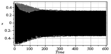
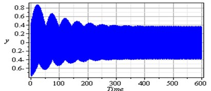
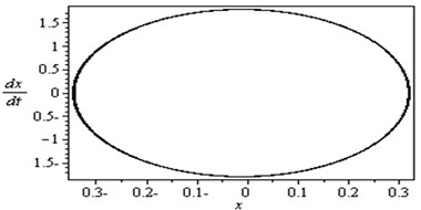
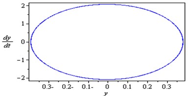
To determine the numerical solution and response of the given system of Eq. (4), the Runge-Kutta of fourth order method was applied. Fig. 2 illustrates the response and the phase-plane for the non-resonant system (basic case) where $γ_{1} \neq γ_{2} \neq γ_{3} \neq γ_{4} \neq ω_{1} \neq ω_{2}$ at some practical values of the equation parameters $μ_{1} = 0.02$ , $β_{1} = 0.03$ , $β_{2} = 0.3$ , $β_{3} = 0.2$ , $β_{4} = 0.05$ , $β_{5} = 0.3$ , $μ_{2} = 0.02$ , $η_{1} = 0.3$ , $η_{2} = 0.03$ , $η_{3} = 0.5$ , $η_{4} = 0.03$ , $η_{5} = 0.3$ , $ρ_{1} = 8.6$ , $ρ_{2} = 8.6$ , $ρ_{11} = 0.02$ , $ρ_{12} = 0.02$ , $ρ_{21} = 0.005$ , $ρ_{22} = 0.005$ , $η_{1} = 0.3$ , $η_{2} = 0.03$ , $η_{3} = 0.5$ , $η_{4} = 0.03$ , $η_{5} = 0.3$ , $ρ_{1} = 8.6$ , $ρ_{2} = 8.6$ , $ρ_{11} = 0.02$ , $ρ_{12} = 0.02$ , $ρ_{21} = 0.005$ , $ρ_{22} = 0.005$ . It is observed from this figure that the response of the first and second modes of the FGM rectangular plate start with increasing amplitude with some chaotic and tuned oscillation respectively, the oscillation of the two modes becomes stable and the steady state amplitudes $x$ and $y$ are about 0.35 and 0.4 respectively and the phase plane shows limit cycle, denoting that the system is free from chaos. Table 1 shows the results of the worst resonance conditions.

Fig. 3 shows that the time response and phase-plane of the simultaneous primary, combined and internal resonance ( $γ_{1} ≅ ω_{1}$ , $γ_{3} - γ_{4} ≅ ω_{1}$ and $ω_{2} ≅ 1 / 2 ω_{1}$ ) which is one of the worst resonance cases. From this figure we have that the amplitude of the first mode of the FGM rectangular plate is increased to about 1950 % of that values shown in Fig. 2, while the amplitude of the second mode is increased to about 1150 % and becomes stable and the phase plane shows multi-limit cycle.

Fig. 3Simultaneous primary combined and internal resonance case: μ1=0.02, β1=0.03, β2=0.3, β3=0.2, β4=0.05, β5=0.3, μ2=0.02, η1=0.3, η2=0.03, η3=0.5, η4=0.03, η5=0.3, ρ1=8.6, ρ2=8.6, ρ11=0.02, ρ12=0.02, ρ21=0.005, ρ22=0.005 ( γ1≅ω1, γ3-γ4≅ω1 and ω2≅1/2ω1)

Simultaneous primary combined and internal resonance case: μ1=0.02, β1=0.03, β2=0.3, β3=0.2, β4=0.05, β5=0.3, μ2=0.02, η1=0.3, η2=0.03, η3=0.5, η4=0.03, η5=0.3, ρ1=8.6, ρ2=8.6, ρ11=0.02, ρ12=0.02, ρ21=0.005, ρ22=0.005 ( γ1≅ω1, γ3-γ4≅ω1 and ω2≅1/2ω1)

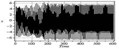
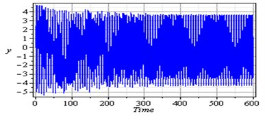
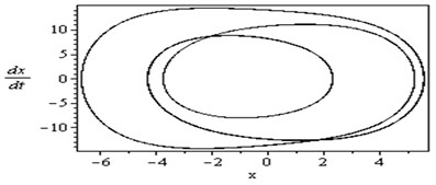
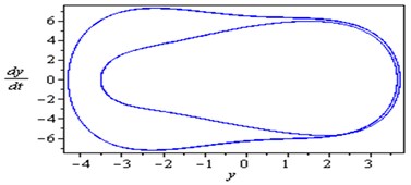
Table 1Summary of the worst resonance cases

Resonance cases	$x$ %	$y$ %	Remarks
Non-resonance case	100 %	100 %	Limit cycle
$γ_{1} ≅ ω_{1}, γ_{1} ≅ ω_{2}, ω_{2} ≅ ω_{1}$	1450 %	1000 %	Multi Limit cycle
$γ_{1} ≅ ω_{1}, γ_{2} ≅ 2 ω_{2}, ω_{2} ≅ ω_{1}$	1450 %	900 %	Multi Limit cycle
$γ_{1} ≅ ω_{1}, γ_{3} - γ_{4} ≅ ω_{2}, ω_{2} ≅ ω_{1}$	1450 %	1000 %	Multi Limit cycle
$γ_{1} ≅ ω_{2}, γ_{2} ≅ 2 ω_{1}, ω_{2} ≅ ω_{1}$	1450 %	900 %	Multi Limit cycle
$γ_{1} ≅ ω_{2}, γ_{3} - γ_{4} ≅ ω_{1}, ω_{2} ≅ ω_{1}$	1450 %	1000 %	Multi Limit cycle
$γ_{1} ≅ ω_{1}, γ_{1} ≅ ω_{2}, γ_{3} - γ_{4} ≅ ω_{1}$	1450 %	1000 %	Multi Limit cycle
$γ_{1} ≅ ω_{1}, γ_{2} ≅ 2 ω_{2}, γ_{3} - γ_{4} ≅ ω_{1}$	1400 %	900 %	Multi Limit cycle
$γ_{1} ≅ ω_{2}, γ_{2} ≅ 2 ω_{1}, γ_{3} - γ_{4} ≅ ω_{1}$	1450 %	800 %	Multi Limit cycle
$γ_{1} ≅ ω_{1}, γ_{3} - γ_{4} ≅ ω_{1}, ω_{2} ≅ 1 / 2 ω_{1}$	1950 %	1150 %	Multi Limit cycle
$γ_{1} ≅ ω_{1}, γ_{3} - γ_{4} ≅ ω_{1}, ω_{2} ≅ 1 / 3 ω_{1}$	1900 %	1100 %	Multi Limit cycle
$γ_{1} ≅ ω_{1}, γ_{3} - γ_{4} ≅ ω_{1}, ω_{2} ≅ 1 / 4 ω_{1}$	1900 %	1100 %	Multi Limit cycle

4.1. Response curves and effects of different parameters

In this section, the steady state response of the given system at various parameters near the simultaneous primary, combined and internal resonance case is investigated and studied. The frequency response equations given by Eq. (26) are solved numerically at the same values of the parameters shown in Fig. 3. In all figures, the solid lines stand for the stable solution and the dashed lines for the unstable solution.

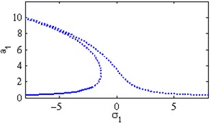
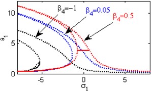
Fig. 4The steady state amplitudes of the first mode of the FGM rectangular plate

a) Effects of the detuning parameter $σ_{1}$

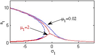
b) Effects of the damping coefficient $μ_{1}$

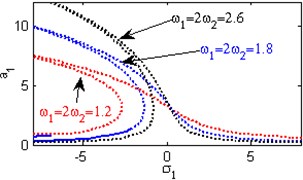
c) Effect of the natural frequencies $ω_{1}$ , $ω_{2}$

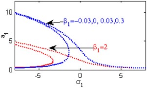
d) Effects of the non-linear parameter $β_{1}$

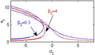
e) Effects of the non-linear parameter $β_{2}$

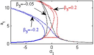
f) Effects of the non-linear parameter $β_{3}$

g) Effects of the non-linear parameter $β_{4}$

h) Effects of the non-linear parameter $β_{5}$

i) Effects of the excitation amplitude $ρ_{1}$

j) Effects of the excitation amplitude $ρ_{21}$

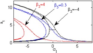
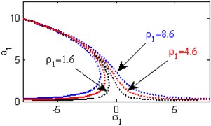
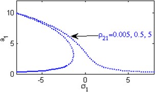
Fig. 4(a) shows the steady state amplitudes of the first mode of the FGM rectangular plate against the detuning parameter $σ_{1}$ at the practical case, where $a_{1} \neq 0$ , $a_{2} \neq 0$ . Fig. 4(b) shows that the steady state amplitude of the first mode of the FGM rectangular plate is a monotonic decreasing function in the linear damping coefficients $μ_{1}$ . Fig. 4(c) show that the steady state amplitude of the first mode is a monotonic decreasing function in the natural frequencies $ω_{1}$ and $ω_{2}$ , in this Figure, the response curve is bent to the right and has harding spring type and there exists jump phenomena. Figs. 4(d), (e) shows that the steady state amplitude of the first mode is a monotonic decreasing function in nonlinear parameter $β_{1}$ , $β_{2}$ and the response curves are bent to the left leading to the occurrence of the jump phenomena and multi-valued amplitudes. The steady state amplitude of the first mode is a monotonic increasing function in the nonlinear parameter $β_{3}$ , $β_{4}$ and the excitation amplitudes $ρ_{1}$ as shown in Figs. 4(f), (g), (i). For increasing value of the nonlinear parameter $β_{5}$ , the amplitude of the first mode is decreased and the curve is shifted to the left as shown in Fig. 4(h). The effect of increasing or decreasing the excitation amplitudes $ρ_{21}$ on the steady state amplitude of the FGM is trivial due to saturation occurrence as shown in Fig. 4(j).

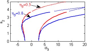
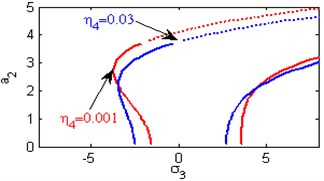
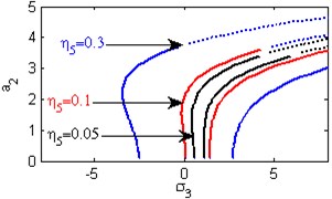
Fig. 5The steady state amplitudes of the second mode of the FGM rectangular plate

a) Effects of the detuning parameter $σ_{3}$

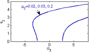
b) Effects of the damping coefficient $μ_{2}$

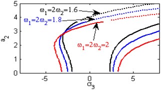
c) Effect of the natural frequencies $ω_{1}$ , $ω_{2}$

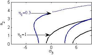
d) Effects of the non-linear parameter $η_{1}$

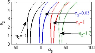
e) Effects of the non-linear parameter $η_{2}$

f) Effects of the non-linear parameter $η_{3}$

g) Effects of the non-linear parameter $η_{4}$

h) Effects of the non-linear parameter $η_{5}$

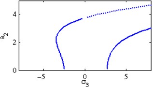
Fig. 5(a) shows the steady state amplitudes of the second mode of the FGM rectangular plate against the detuning parameter $σ_{3}$ at the practical case, where $a_{1} \neq 0$ , $a_{2} \neq 0$ . In this Figure, the response amplitude consists of a continuous curve which is bent to the right and there exists jump phenomena. Fig. 5(b) shows that the effect of increasing or decreasing the linear damping coefficients $μ_{2}$ on the steady state amplitude of the second mode of FGM is trivial due to saturation occurrence. Figs. 5(c), (d), (f), (g) show that the steady state amplitude of the second mode is a monotonic decreasing function in nonlinear parameter $η_{1}$ , $η_{3}$ , $η_{4}$ and the natural frequencies $ω_{1}$ , $ω_{2}$ and the response curves are bent to the right leading to the occurrence of the jump phenomena and multi-valued amplitudes. For increasing value of the nonlinear parameter $η_{2}$ , the amplitude of the second mode is shifted to the right as shown in Fig. 5(e). The steady state amplitude of the first mode is a monotonic increasing function in the nonlinear parameter $η_{5}$ _,as shown in Fig. 5(h).

4.2. Comparison between the numerical and analytical simulation

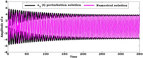
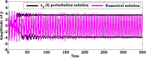
Fig. 6Comparison between numerical solution (using RKM) and analytical solution (using perturbation method) of the system at ρ1=8.6, ρ2=8.6

a)

b)

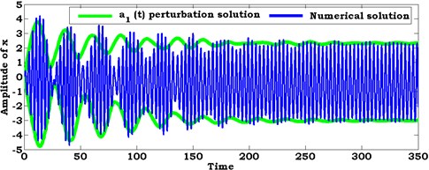
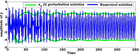
Fig. 7Comparison between numerical solution (using RKM) and analytical solution (using perturbation method) of the system at ρ1=1.6, ρ2=1.6

a)

b)

In this section, the system of nonlinear differential equations given by Eqs. (21) and (22) are solved numerically at the simultaneous primary, combined and internal resonance case where $γ_{1} ≅ ω_{1}$ , $γ_{3} - γ_{4} ≅ ω_{1}$ and $ω_{2} ≅ 1 / 2 ω_{1}$ . Figs. 6 and 7 show the comparison between numerical integration for the system Eqs. 4(a), (b) and the amplitude-phase modulating Eqs. (21) and (22) at different values of excitation force amplitudes $ρ_{1}$ and $ρ_{2}$ . We found that all predictions from analytical solutions are in good agreement with the numerical simulation.

5. Conclusions

Multiple time scale perturbation method is useful to determine approximate solutions for the coupled nonlinear differential equations describing the FGM rectangular plate system up to and including the second order approximation. Both the frequency response equations and the phase-plane technique are applied to study the stability of the system. The effect of the different parameters of the system is studied numerically. From the above study the following may be concluded:

1) The amplitude of the first mode FGM rectangular plate is increased to about 0.35, while the amplitude of the second mode is increased to about 0.4 at the non-resonant case ( $γ_{1} \neq γ_{2} \neq γ_{3} \neq γ_{4} \neq ω_{1} \neq ω_{2}$ ).

2) The amplitude of the first mode FGM rectangular plate is increased to about 1950 % of that values shown in Fig. 2, while the amplitude of the second mode is increased to about 1150 % at the worst resonance case (the simultaneous primary, combined and internal resonance $γ_{1} ≅ ω_{1}$ , $γ_{3} - γ_{4} ≅ ω_{1}$ and $ω_{2} ≅ 1 / 2 ω_{1}$ ).

3) The amplitude of the first and second mode FGM rectangular plate are increased to about 1900 % and 1100 % respectively at the worst resonance case ( $γ_{1} ≅ ω_{1}$ , $γ_{3} - γ_{4} ≅ ω_{1}$ and $ω_{2} ≅ 1 / 3 ω_{1}$ ) and ( $γ_{1} ≅ ω_{1}$ , $γ_{3} - γ_{4} ≅ ω_{1}$ and $ω_{2} ≅ 1 / 4 ω_{1}$ ).

4) The steady state amplitudes of the FGM rectangular plate are a monotonic decreasing function the linear damping coefficients $μ_{1}$ , the nonlinear parameters ( $β_{1}$ , $β_{2}$ , $β_{5}$ , $η_{1}$ , $η_{3}$ , $η_{4}$ ) and the natural frequencies $ω_{1}$ and $ω_{2}$ .

5) The steady state amplitudes of FGM rectangular plate are a monotonic increasing function in the nonlinear parameters ( $β_{3}$ , $β_{4}$ , $η_{5}$ ) and the excitation amplitude $ρ_{1}$ .

6) The effects of increasing or decreasing the linear damping coefficients $μ_{2}$ and the excitation amplitude $ρ_{21}$ on the steady state amplitude of the FGM are trivial due to saturation occurrence.

7) The analytical solutions are in good agreement with the numerical simulation at different values of excitation amplitude forces $ρ_{1}$ and $ρ_{2}$ .

References

Reddy J. N., Cheng Z. Q. Three-dimensional thermomechanical deformations of functionally graded rectangular plates. European Journal of Mechanics, Vol. 20, 2001, p. 841-855.

Search CrossRef
Reddy J. N. Analysis of functionally graded plates. International Journal of Numerical Methods Engineering, Vol. 47, 2000, p. 66 3-684.

Search CrossRef
Yang J., Kitipomchai S., Liew K. M. Large amplitude vibration of thermo-electro mechanically stressed FGM laminated plates. Computer Methods in Applied Mechanics and Engineering, Vol. 192, 2003, p. 3861-3885.

Search CrossRef
Huang X. L., Shen H. S. Nonlinear vibration and dynamic response of functionally graded plates in thermal environments. International Journal of Solids and Structures, Vol. 41, 2004, p. 2403-2407.

Search CrossRef
Kitipornchai S., Yang J., Liew M. K. Semi-analytical solution for nonlinear vibration of laminated FGM plates with geometric imperfections. International Journal of Solids and Structures, Vol. 41, 2004, p. 2235-2257.

Search CrossRef
Yang J., Huang X. L. Nonlinear transient response of functionally graded plates with general imperfections in thermal environments. Computer Methods in Applied Mechanics and Engineering, Vol. 196, 2007, p. 2619-2630.

Search CrossRef
Ye M., Lu J., Zhang W., Ding Q. Local and global nonlinear dynamics of a parametrically excited rectangular symmetric cross-ply laminated composite plate. Chaos Solitons and Fractals, Vol. 26, 2005, p. 195-213.

Search CrossRef
Haddadpour H., Navazi H. M., Shadmehri F. Nonlinear oscillations of a fluttering functionally graded plate. Composite Structure, Vol. 79, 2007, p. 242-250.

Search CrossRef
HaoY. X., Chen L. H., Zhang W., Lei J. G. Nonlinear oscillations, bifurcations and chaos of functionally graded materials plate. Journal of Sound and Vibration, Vol. 312, 2008, p. 862-892.

Search CrossRef
Zhang W., Yang J., Hao Y. X. Chaotic vibrations of an orthotropic FGM rectangular plate based on third-order shear deformation theory. Nonlinear Dynamics, Vol. 59, 2010, p. 619-660.

Search CrossRef
Yang J., Hao Y. X., Zhang W., Kitipornchai S. Nonlinear dynamic response of a functionally graded plate with a through-width surface crack. Nonlinear Dynamics, Vol. 59, 2010, p. 207-219.

Search CrossRef
Li S. B., Zhang W., Hao Y. X. Multi-pulse chaotic dynamics of a functionally graded material rectangular plate with one-to-one internal resonance. International Journal of Nonlinear Science and Numerical Simulation, Vol. 11, 2010, p. 351-362.

Search CrossRef
Malekzadeh P., Golbahar Haghighi M. R., Atashi M. M. Free vibration analysis of elastically supported functionally graded annular plates subjected to thermal environment. Meccanica, Vol. 46, Issue 5, 2011, p. 893-913.

Search CrossRef
Akbarzadeh A. H., Abbasi M., Hosseini S. K., Eslami M. R. Dynamic analysis of functionally graded plates using the hybrid Fourier-Laplace transform under thermomechanical loading. Meccanica, Vol. 46, Issue 6, 2011, p. 1373-1392.

Search CrossRef
Zhang W., Hao Y., Guo X., Chen L. Complicated nonlinear responses of a simply supported FGM rectangular plate under combined parametric and external excitations. Meccanica, Vol. 47, 2012, p. 985-1014.

Search CrossRef
Eissa M., Sayed M. A comparison between passive and active control of non-linear simple pendulum Part-I. Mathematical and Computational Applications, Vol. 11, 2006, p. 137-149.

Search CrossRef
Eissa M., Sayed M. A comparison between passive and active control of non-linear simple pendulum Part-II. Mathematical and Computational Applications, Vol. 11, 2006, p. 151-162.

Search CrossRef
Eissa M., Sayed M. Vibration reduction of a three DOF non-linear spring pendulum. Communication in Nonlinear Science and Numerical Simulation, Vol. 13, 2008, p. 465-488.

Search CrossRef
Hamed Y. S., El-Ganaini W. A., Kamel M. M. Vibration suppression in ultrasonic machining described by non-linear differential equations. Journal of Mechanical Science and Technology, Vol. 23, Issue 8, 2009, p. 2038-2050.

Search CrossRef
Hamed Y. S., EL-Ganaini W. A., Kamel M. M. Vibration suppression in multi-tool ultrasonic machining to multi-external and parametric excitations. Acta Mechanica Sinica, Vol. 25, 2009, p. 403-415.

Search CrossRef
Hamed Y. S., El-Ganaini W. A., Kamel M. M. Vibration reduction in ultrasonic machine to external and tuned excitation forces. Applied Mathematical Modeling, Vol. 33, 2009, p. 2853-2863.

Search CrossRef
Sayed M., Hamed Y. S. Stability and response of a nonlinear coupled pitch-roll ship model under parametric and harmonic excitations. Nonlinear Dynamics, Vol. 64, 2011, p. 207-220.

Search CrossRef
Hamed Y. S., Sayed M., Cao D.-X., Zhang W. Nonlinear study of the dynamic behavior of a string-beam coupled system under combined excitations. Acta Mechanica Sinica, Vol. 27, Issue 6, 2011, p. 1034-1051.

Search CrossRef
Sayed M., Hamed Y. S., Amer Y. A. Vibration reduction and stability of non-linear system subjected to external and parametric excitation forces under a non-linear absorber. International Journal of Contemporary Mathematical Sciences, Vol. 6, Issue 22, 2011, p. 1051-1070.

Search CrossRef
Amer Y. A., Sayed M. Stability at principal resonance of multi-parametrically and externally excited mechanical system. Advances in Theoretical and Applied Mechanics, Vol. 4, 2011, p. 1-14.

Search CrossRef
Sayed M., Kamel M. Stability study and control of helicopter blade flapping vibrations. Applied Mathematical Modelling, Vol. 35, 2011, p. 2820-2837.

Search CrossRef
Sayed M., Kamel M. 1:2 and 1:3 internal resonance active absorber for non-linear vibrating system. Applied Mathematical Modelling, Vol. 36, 2012, p. 310-332.

Search CrossRef
Sayed M., Mousa A. A. Second-order approximation of angle-ply composite laminated thin plate under combined excitations. Communication in Nonlinear Science and Numerical Simulation, Vol. 17, 2012, p. 5201-5216.

Search CrossRef
Sayed M., Mousa A. A. Vibration, stability, and resonance of angle-ply composite laminated rectangular thin plate under multi excitations. Mathematical Problems in Engineering, Vol. 2013, 2013, p. 1-26.

Search CrossRef
Reddy N. A refined nonlinear theory of plates with transverse shear deformation. International Journal of Solids and Structures, Vol. 20, Issue 9-10, 1984, p. 881-896.

Search CrossRef

About this article

Received

03 December 2013

Accepted

20 June 2014

Published

15 November 2014

Keywords

FGM rectangular plate

vibrations

chaotic dynamics

stability

saturation

Acknowledgements

The author would like to thank the anonymous reviewers for their valuable comments and suggestions for improving the quality of this paper.

This is an open access article distributed under the Creative Commons Attribution License, which permits unrestricted use, distribution, and reproduction in any medium, provided the original work is properly cited.