Mean change-point model for aero-engine component faults

Fu, Yu; Zuo, Hongfu; Cai, Jing; Yin, Yibing

Journal of Vibroengineering

Browse Journal

Submit article

Published: 31 December 2013

Check for updates

Mean change-point model for aero-engine component faults

Yu Fu¹

Hongfu Zuo²

Jing Cai³

Yibing Yin⁴

^{1, 2, 3, 4}College of Civil Aviation, Nanjing University of Aeronautics and Astronautics, P. R. China

Corresponding Author:

Yu Fu

Cite the article Download PDF

Downloads 1057

Abstract

Recognizing aero-engine component faults is important in prognostics and health management research, particularly in engine monitoring systems and condition-based maintenance. The former primarily concentrates on recognizing engine working parameters and component performance, and neglects quantitative changes in component faults. Taking lubricating oil consumption as an example, quantitative changes in component faults are analyzed using a mean change-point model based on change-point theory. The change-point stage is presented through the minimum variance algorithm. The change point corresponding to the failure mode is tested using exhaust electrostatic data from a turbojet engine life span experiment to verify the validity and feasibility of the theory.

1. Introduction

Ensuring flight safety through accurate and timely monitoring of aero-engine working state is a significant precondition. Recognizing aero-engine component faults is important in prognostics and health management [1] research, particularly in engine monitoring systems and condition-based maintenance [2]. The former primarily concentrates on recognizing analytical relationships between component parameters and performance [3-8], and neglects quantitative changes in component states. Quantitative changes are preconditions and provisions for qualitative changes, and qualitative changes increase with increasing quantitative changes [9]. Accordingly, quantitative changes should be studied for real-time recognition of engine working state. Change-point theory [10] has been recently developed to study quantitative changes in nonlinear statistical theory. Based on the mean change-point algorithm, the change point is found to exist with lubricating oil consumption (OC) data. In addition, real-time data from electrostatic sensors are collected to verify corresponding faults and to determine whether the engine is abnormal.

2. Presentation of change-point model

Change point is ubiquitous in nature and in the social fields. It reflects changes in inherent law and in the process involved in the transformation of quantitative to qualitative changes. The change point is generally the aspect that suddenly changes in a certain model. This problem comprises a series of observed values (samples). In most cases, these values are arranged in chronological order. The point at which the distribution or statistical characteristics of samples suddenly change is called the change point. In addition, sample distribution is dependent on spatial parameters. The change point is the position in space or interface. It is equal to the time variable in one-dimensional space.

3. Oil consumption change-point model

3.1. Mean change-point model

Mean change-point model, which is feasible and convenient in practical applications, is applied in this study. Supposing $X$ is the lubricating OC per hour, $X_{t} = a_{t} + e_{t}$ ; $t = 1, 2, \dots, N$ ; $a_{1} = a_{m 1 - 1 \dots} = b_{1}$ ; $a_{m 1} = a_{m 2 - 1 \dots} = b_{2}$ ; $a_{m q} = \dots = a_{n \dots} = b_{q + 1}$ ; $1 < m_{1} < m_{2} < \dots < m_{q} < n$ . $m_{j}$ is the change point. $e_{1}, e_{2}, \dots, e_{n}$ is the random error of the model.

3.2. Minimum variance method to change point

Whether the change point exists, that is:

Original hypothesis $H_{0}$ : $b_{1} = b_{2} = \dots = b_{q + 1}$ .

If $H_{0}$ is accepted, a change point does not exist.

If $H_{0}$ is rejected, at least one change point exists in the data sequence. The data sequence contains $q$ point. Accordingly, change points $m_{1}, m_{2}, \dots, m_{q}$ can be estimated.

The small probability principle was applied to this hypothesis testing. The allowable small probability, which was judged as the boundary before identification, was at significance level $α$ . In statistics, $α$ stands for the size of I-type error. That is, if the original hypothesis is accepted, $α$ is the rejection probability. In this study, the significant level $α$ is 0.05, and the corresponding confidence interval is 95 %.

OC: $X_{1}, X_{2}, \dots, X_{N}$ is independent from each other; $t$ is the time interval per unit. The following are the steps for the minimum variance method of searching for change points.

(1) With $i = 2, \dots, N$ , the sample is divided into two sections: $X_{1}, X_{2}, \dots, X_{i - 1}$ and $X_{i}, X_{i + 1}, \dots, X_{N}$ . Then, the arithmetic mean values ${\bar{X}}_{i 1}$ , ${\bar{X}}_{i 2}$ and the statistics of each sample section are calculated as follows:

1

S_{i} = \sum_{t = 1}^{i - 1} (x_{t} - {\bar{X}}_{i 1})^{2} + \sum_{t = i}^{N} (x_{t} - {\bar{X}}_{i 2})^{2} .

(2) Calculating the statistics is as follows:

2

\bar{X} = \sum_{t = 1}^{N} x_{t} / N, and S = \sum_{t = 1}^{N} {(x_{t} - \bar{X})}^{2} .

(3) Calculating the expected value is as follows:

3

E (S - S_{i}) = E (N^{- 1} (i - 1) (N - i + 1) {({\bar{X}}_{i 1} - {\bar{X}}_{i 2})}^{2}) = σ^{2} + N^{- 1} (i - 1) (N - i + 1) {(E {\bar{X}}_{i 1} - E {\bar{X}}_{i 2})}^{2}, i = 2, 3, . . ., N .

(4) Calculating the maximum value is as follows:

4

E (S - S^{*}) = \underset{2 \leq i \leq N}{m a x} E (S - S_{i}),

where $S^{*} = m i n (S_{2}, . . ., S_{N}) .$

(5) Taking $α$ as the significant level of inspection, the value of $C$ is calculated [10].

The following can be obtained using probability limit theorems:

5

\underset{n \to \infty}{l i m} P (\frac{S - S^{*}}{σ^{2}} < 2 l n l n n + l n l n l n N - l n π + z) = \exp (- 2 e^{- \frac{z}{2}}) .

If sigma-squared is known for the given $α > 0$ , then $\exp (- 2 e^{- \frac{z}{2}}) = 1 - α$ . The solution is as follows:

6

C = σ^{2} (2 l n l n N + l n l n l n N - l n π - 2 \ln (- 0.5 \ln (1 - α))) .

If sigma-squared is unknown in the preceding equation, then the estimation is conducted as follows:

7

{\hat{σ}}^{2} = S^{*} / (N - 2 l n l n N - l n l n l n N - 2.4) .

(6) If $S - S^{*} > C$ , $H_{0}$ is negative, i.e., a change point exists; otherwise, $H_{0}$ is accepted.

For simplicity, $q = 1$ in this study. This change point can be estimated from Equations (1) to (7), and the change point estimated value of OC $\hat{m}$ is the corresponding value $i$ of $S^{*}$ .

4. Model applications

4.1. Data source

Data came from an aviation turbojet engine [11]. The experimental engine was tested for a life span of 200 h in July 2011, and data were collected during the 200 h life span test (an additional 40 h was provided after the 200 h, giving a total of 240 h), with each test having 1 h per stage. Figure 1 shows OC data from stages 95 to 117, and in this paper $N =$ 23. These data were tested using the change-point algorithm, whereas electrostatic data were obtained to analyze and verify the change point.

Fig. 1Lubrication oil consumption from stages 95 to 117

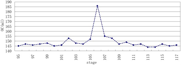
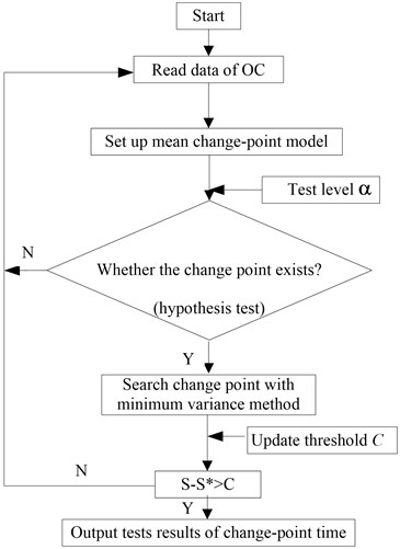
Fig. 2The searching flowchart

4.2. Algorithm process

The change point with the algorithm is shown in the minimum variance method, and the flowcharts are shown in Fig. 2.

4.3. Experimental results

The test level $α$ was set to 0.05 in the simulation. The results show a change point in OC in the 106th stage according to the algorithm and searching flowchart (Table 1).

Table 1Test results of the change point

Average OC on the change point (ml)	$α$	$S$	$S^{*}$	$C$	Change point time	$S - S^{*} > C$ (Y/N)
186	0.05	1188.222	1187.564	0.374	106th stage	Y

The average OC was 186 ml within the 106th time interval. A lubricating oil leakage fault was speculated. Inspection revealed oil leakage at the starter generator. After replacing the sealing ring and reinstalling the starter generator, the 107th stage was started for testing. OC obviously decreased, and the test results of the change point corresponded with the actual condition.

4.4. Verification tests

4.4.1. Electrostatic statistical signals

Electrostatic statistical signals were analyzed to describe the correctness of change-point testing and to distinguish differences between normal signals and gas oil leakage fault signals when oil data changed. Electrostatic data were used to detect electrostatic particles in engine exhaust [12-14]. The principle states that abnormal particles are engendered in excessive oil leakage, rubbing, and other anomalies in gas path components. These abnormal particles change the level of charged particles in the gas path.

Data came from an aviation turbojet engine. The experimental engine started to test for 200 h life span in July 2011, and the data were carried out during the 200 h life span test (there were an additional 40 hours after 200 h, totally 240 hours), each test 1 h as a stage.

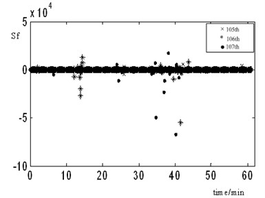
In the present test, the 105th, 106th, and 107th stages represent the normal signal, fault signal, and the signal after fault exclusion, respectively. In addition, the root mean square (RMS), clearance factor (CLf), impulsion factor (If), and signal waveform factor (Sf) were discussed. These parameters were more sensitive to electrostatic signal fault in time domain. The calculation results are shown in Figs. 3 to 6.

Fig. 3The RMS of electrostatic signals

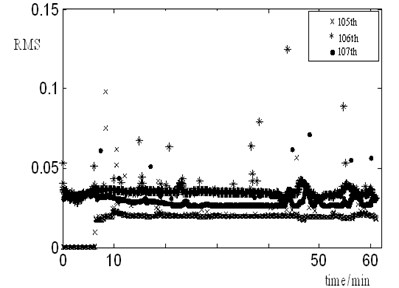
Fig. 4The CLf of electrostatic signals

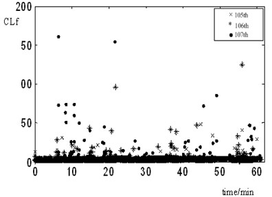
Fig. 5The If of electrostatic signals

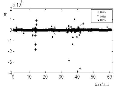
Fig. 6The Sf of electrostatic signals

Under normal working conditions, the base line of the time-domain signal was maintained at the millivolt level, and the normal charge of particles was 0.3 pc to 0.5 pc. The abnormal pulse emerged within the 106th stage of the test; V-level signals even appeared. In addition, the activity level of the 106th stage appeared relatively larger. The activity level was the effective value of the induction charge at a certain time interval. The activity level changed simultaneously with oil leakage. The activity level from the 95th to 105th stages went steadily; however, that in the 106th stage significantly increased, along with a large number of outliers. After troubleshooting, activity levels declined.

Event rate indicates larger particles in the gas exhaust (greater than 40 micron particles). According to the polarity difference in charged particles, event rate can either be positive or negative. A positive event rate denotes non-metallic particles, whereas a negative event rate represents large metal particles. Several positive event rate points appeared in the 106th stage, thus indicating the presence of large non-metallic particles. This finding could be attributed to the improper installation of the engine starting motor, which resulted in lubricating oil leakage in the gas path. The oil was inhaled into the combustion chamber with high-temperature air. A negative effect was exerted on combustion performance. Meanwhile, a negative event rate remained at approximately 2 %, with almost no abnormal metal particle.

The RMS stands for signal average power in unit time. Figure 3 shows that the electrostatic signal RMS in the 106th stage is greater than that in the 107th and 105th stages. Moreover, the RMS in the 107th stage is slightly greater than that in the 105th stage. This finding indicates that oil leakage in the gas path increases RMS signal. After troubleshooting, the effects of the faults are difficult to eliminate within a short period.

CLf, If and Sf were introduced to represent the characteristics of failures and to express the change-point pulse of the electrostatic signals. Figures 4 to 6 show that the frequency and number of abnormal points in CLf, If and Sf appeared analogously in the 106th and 107th stages. These statistical parameters of the signals indicate that early faults occurred in these stages, which were different from the normal electrostatic signal in the 105th stage. In fact, although the change point occurred in the 106th stage, the residual oil particles in the gas path must have resulted in abnormal points in the 107th stage.

4.4.2. SPSS statistical analysis

The statistical analysis by SPSS [15] have confirmed the assumed conditions of Gaussian law and relationship between OC and electrostatic particles in the flow. Taking electrostatic signal data as dependent variable, oil consumption as variable, regression analysis is established by SPSS, results are given as in Table 2 and 3.

Model 1 indicates the regression model formed by electrostatic signal data ( $E$ ) and oil consumption (OC). The value of Adjusted $R_{2}$ is 0.865, nearly 1, which indicates the fitting degree of model 1 is acceptable. Moreover, the Durbin-Watson value is 1.947, nearly 2, thus, random error $e_{i}$ is independent.

Table 2Model correlation description and residual series independence tests

Model	$R$	$R^{2}$	Adjusted $R^{2}$	Durbin-Watson
1	0.934	0.871	0.865	1.947

Table 3Residuals statistics

	Minimum	Maximum	Mean	N
Predicted Value	-2.0840	19.8487	1.1094	23
Residual	-3.55687	2.85132	0.00000	23
Std. Predicted Value	-0.723	4.244	0.000	23
Std. Residual	-2.050	1.643	0.000	23

From Table 3, both mean residual and mean standard residual was 0.000 in residuals statistics, thus indicating that the residual distribution satisfies the zero mean assumption, i.e., $E (e_{i}) = 0$ .

5. Conclusions

OC with its quantity change point occurring time is analyzed according to actual aero-engine test data. Combined with change-point theory and advanced electrostatic induction technology, the change point corresponding to the failure mode is verified. The conclusions are given as follows.

(1) Searching for change points can effectively detect quantitative change occurring time of component states, which can be considered as advanced monitoring before qualitative faults. Based on the aforementioned algorithm, any abnormality in engine working condition can be detected early for condition-based maintenance.

(2) The results exhibited a change point for OC in the 106th stage during the life span test. After the 106th commissioning, an obvious oil trace was found in the path inlet. Engineers inferred the presence of oil leakage on the sealed portion of the starter generator. After replacing the sealing ring and reinstalling the starter generator, OC decreased in the 107th stage, and the fault was eliminated.

(3) Electrostatic induction signal confirmed the presence of a corresponding fault. Although the electrostatic pulse signal appeared in the 106th stage and in other stages, differences in pulse amplitude, time (more than 0.5 V pulse, for example), and emerging time were observed. The pulse maximum amplitude in the 106th stage was 3.25 V, thus demonstrating oil leakage.

(4) Electrostatic signal fault characteristics of lubricating oil leakage showed that the RMS value in the 106th stage of the change point was higher. In addition, the frequency and number of abnormal points in CLf, If, and Sf appeared frequently in the 106th stage, thus suggesting that early faults occurred in this stage. Although OC was decreased, abnormal points still occurred in CLf, If, and Sf because the effects of faults (i.e., residual oil particles in the gas path) were difficult to eliminate within a short period. As a result, abnormal points appeared in the 107th stage.

References

Guo Yangming, Cai Xiaobin, Zhang Baozhen. Review of prognostics and health management technology. Computer Measurement & Control, Vol. 16, Issue 9, 2008, p. 1213-1216.

Search CrossRef
Roemer M. J., Kacprzynski G. J., Schoeller M. H. Improved diagnostic and prognostic assessments using health management information fusion. IEEE Systems Readiness Technology Conference, Valley Forge, PA, 2001, p. 365-377.

Search CrossRef
Hui Yu, Hongfu Zuo, Chuanqi Huang. Advanced endoscopy and fault testing of aeronautic engine. Aviation Engineerging & Maintenance, 2002, p. 20-22.

Search CrossRef
Fiorucci T. R., Iakin D. R., Reynolds T. D. Advanced engine health management applications of the SSME real-time vibration monitoring system. 36th AIAA/ASME/SAE/ASEE Joint Propulsion Conference, AIAA-2000-3622, 2000.

Search CrossRef
Blazowski W. S. Dependence of soot production on fuel blend characteristics and combustion conditions. Journal of Engine Power, Vol. 102, Issue 2, 1980, p. 403-408.

Search CrossRef
Lawen J. L., Flower G. T. Interaction dynamics between a flexible rotor and an auxiliary clearance bearing. ASME Journal of Vibration and Acoustics, Vol. 121, 1999, p. 183-189.

Search CrossRef
Grapis O., Tamuzs V. Overcritical high-speed rotor systems, full annular rub and accident. Journal of Sound and Vibration, Vol. 290, 2006, p. 910-927.

Search CrossRef
Dowson P., Walker M. S., Watson A. P. Development of abradable and rub-tolerant seal materials for application in centrifugal compressors and steam turbines. Sealing Technology, 2004, p. 5-10.

Search CrossRef
Fu Yu, Wang Xiaoyuan. Binary linear regression change-point identification method of the traffic flow based on projection transformation. Computer Applications, Vol. 30, Issue 1, 2010, p. 263-265, 279.

Search CrossRef
Xiang Jingtian, Shi Jiuen. Statistical Methods Dealing with Data in Non-Linear System. Science Press, Beijing, 2000.

Search CrossRef
Yu Fu, Hongfu Zuo, Ruiming Wang. A monitoring experiment for gas path electrostatic probe-type sensor on turbojet engine. Information Technology Journal, Vol. 12, Issue 2, 2013, p. 331-337.

Search CrossRef
Powrie H., Novis A. Gas path debris monitoring for F-35 joint strike fighter propulsion system PHM. Proceedings of IEEE Aerospace Conference, Montana, USA, 2006, p. 1-8.

Search CrossRef
Wen Zhenhua, Zuo Hongfu, Daniel Kit Lau, et al. Research on electrostatic monitoring technology for aero-engine gas path. Prognostics and Health Management Conference, Macao, 2010, p. 1-5.

Search CrossRef
Li Yaohua, Zuo Hongfu, Liu Pengpeng. Gas path electrostatic monitoring of turbo-shaft engine: an exploratory experiment. Acta Aeronautica Et Astronautica Sinica, Vol. 31, Issue 11, 2010, p. 2174-2181.

Search CrossRef
Haijie Y., ErL. SPSS 15.0 for Windows. A Brief Introduction. Social Sciences Academic Press, Beijing, China, 2008.

Search CrossRef

About this article

Received

16 May 2013

Accepted

19 August 2013

Published

31 December 2013

Keywords

turbojet engine

condition-based maintenance

change-point recognition

oil malfunction

Acknowledgements

This research was performed under Doctoral Fellowship, which is funded by National Natural Science Foundation of China (No. 60939003) and partly supported by Natural Science Fund Project in Jiangsu Province (BK2011737). The authors thank them for their financial support.

This is an open access article distributed under the Creative Commons Attribution License, which permits unrestricted use, distribution, and reproduction in any medium, provided the original work is properly cited.