Abstract
This article describes a simple and easy to implement method for numerical computing of movement of general multibody mechanism. The method is suitable for two or three-dimensional space, rigid bodies and all types of kinematic joints. The main advantage of this method lies in the possibility of using very low discretization time step but with high computing performance due effective implementation. This approach has a positive effect to numerical stability, speed and resistance to discontinuous parameter changes. The usability of described method is verified through an experimental multibody system.
1. Introduction
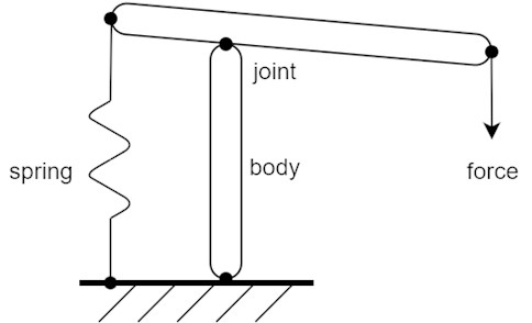
Numerical solution of moving objects is an important theme, especially for mechanism simulations. These simulations are solved with applications called multi-body systems, where mechanisms Fig. 1 are assembled from rigid bodies, kinematic linkages, and other force interaction elements (e.g. external forces, springs, dampers, etc.). The method of solution described above is suitable for use in a computing environment of multibody systems.
Fig. 1Schematic mechanism made up of rigid bodies, kinematic joints, spring and outer force
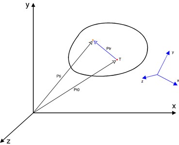
For the purposes of this article, only the solution to determine the body movements if all acting forces are known is going to be discussed. This kind of body Fig. 2 can be defined as absolutely rigid, with non-zero and positive weight and with main moments of inertia. These values are related to the body’s center of gravity. Furthermore, the body may contain other general points whose position is, again, determined relatively to the position of the body’s center of gravity. Each common point of the body is therefore represented by their own local coordinate system (LCS), while the position and orientation of the body itself, i.e. its center of gravity, will be determined in the global coordinate system (GCS).
Each of the points can be used, for example, as an acting place of external forces or moments, references for kinematic constraints, kinematic sensors, etc.
1.1. Body movement
The position of each object in GCS can be defined using the two data structures, where the first is a vector specifying displacement of the body’s center of gravity to the GCS origin, and the second is the transformation matrix for transformation from the local body space to the global space. For description of the rotation (i.e. orientation) the transformation matrix C for rotation around the general axis Eq. (1) is used [1]:
where ex, ey and ez are the unit direction vector components of the general axis of rotation and θ is the angle of rotation.
The movement of body is then in each iteration determined by the Newton-Euler equations of motion. In the environment of the multibody system, the entire solution could be as follows:
1) Determining of the force and torque results in the center of gravity.
2) Updating the kinematic state of the center of the gravity.
3) Updating the kinematic state of other common points of the body.
1.2. Force and torque results of body
Points of the body Fig. 2 are indexed from zero to N-1, where n is the number of points. The first point (i.e. point with zero index) is the body’s center of gravity.
Fig. 2A body in global and local coordinate system (highlighted)
Force and torque resultants in the body’s center of gravity Eqs. (2-3) are determined as a vector sum of the forces and moments in all of the points of the body. If gravitational acceleration is acting on the body, it can also be included in the resultant equations Eq. (2):
1.3. Kinematic state in the center of gravity
Body’s kinematic state, or its center of the gravity, is determined by the Newton-Euler motion equations. Translational component arises from classical Newtonian motion Eq. (4), the velocity and position is obtained by subsequent integration Eqs. (5-6):
Angular acceleration Ar is determined on the basis of Euler’s motion equation Eq. (7), where it is necessary to transform torque vector Mcg and angular velocity vector Vr using transformation matrix C to the local coordinate system of the body (determined by orientation of the center of the gravity), and then the result is transformed back to the global coordinate system [2]. It is because of the correct calculation of the inertia tensor which is, in contrast to the weight, directional. Angular velocity Vr is determined by simple integration of angular acceleration Eq. (8):
To obtain the orientation of the body, which is represented by the transformation matrix of rotation around the arbitrary axis Eq. (2), is not possible to use integration of the velocity vector in a three-dimensional space, as with the translational movement (this is possible only in a plane) However, it is necessary to utilize a matrix process to compose rotations. In the form working with the discretization step Δt, the calculation then has following form: first, the angular velocity vector Vr Eq. (8) is determined after the normalization of the direction of rotation axis e Eq. (9) and by using the discretization step it is possible to compute the appropriate angle of rotation θ Eq. (10):
Subsequently, by using the transformation matrix Eq. (1) the incremental transformation matrix is calculated, and by multiplying it with matrix of rotational position from the previous discretization step the new rotational position for actual time is determined Eq. (11):
1.4. Kinematic state of common points
After the kinematic state of center of the gravity is calculated, all of other kinematic states in the remaining points of the body can be easily determined. The translational position of the point in GCS is determined by transformation and addition of relative displacement vector to the translational position of the center of gravity Eq. (12). Vectors of translational velocity and accelerations are calculated as the numerical derivation of positions, or acceleration Eqs. (14-16). Orientation (i.e. “rotational position”) is the product of a transformation matrix of the center of gravity and the transformation matrix in the relevant point Eq. (13). Angular acceleration and angular velocity of all points of the body are identical, so their values can be determined directly from point 0 Eqs. (15-17), which were determined when calculating the kinematic state of the body’s center of gravity of the body :
2. Conclusions
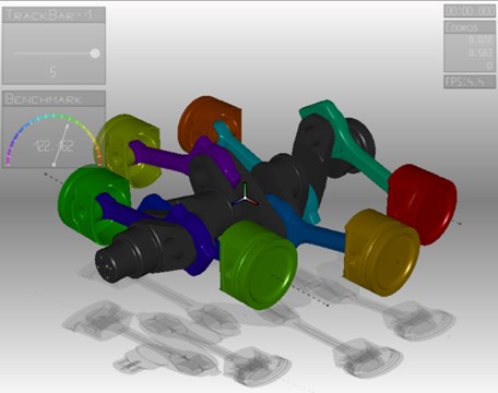
The method described in this article provides a simple and reliable approach to numerical solution of motion of bodies in three-dimensional space Fig. 3. Using the transformation matrix for rotation around the arbitrary axis, elegantly avoids the problems arising from the composition of rotations in space. The advantages are also easy and straightforward implementations using conventional programming languages, type C, Pascal, Matlab, etc. This method is designed to use a very small-time step in range of 10-5 to 10-7 seconds for common mechanism. In this case the numerical solution does not require any complex numerical solvers. Thanks to this, the resulting program code is short, memory transfers are minimized and all executing loops are very tight, which brings high and stable performance. Mechanisms composed of dozens of bodies, kinematic joints and other objects can be simulated in real time on an average computer.
Fig. 3Multibody system based on described method
References
-
Zháňal L. Simulation of Kinematics and Dynamics of Vehicle Mechanisms. Brno University of Technology, Brno, 2015, (in Czech).
-
Porteš P. Using Mathematical Vehicle Models to Analyze Measured Data. Brno University of Technology, Brno, 2015, (in Czech).
About this article

The research leading to these results has received funding from the MEYS under National Sustainability Programme I (Project LO1202) and Specific Research Project of the Faculty of Mechanical Engineering, Brno University of Technology (FSI-S-17-4104).
