Vibrations of the nonlinear system in which stationary harmonic excited multivalued regimes in the vicinities of resonances do not exist

Ragulskis, K.; Ragulskis, L.

doi:10.21595/mme.2019.20942

Mathematical Models in Engineering

Browse Journal

Submit article

Published: 30 September 2019

Check for updates

Vibrations of the nonlinear system in which stationary harmonic excited multivalued regimes in the vicinities of resonances do not exist

K. Ragulskis¹

L. Ragulskis²

¹Kaunas University of Technology, K. Donelaičio Str. 73, LT-44249, Kaunas, Lithuania

²Vytautas Magnus University, Vileikos Str. 8, LT-44404, Kaunas, Lithuania

Corresponding Author:

K. Ragulskis

Cite the article Download PDF

Downloads 1175

Abstract

A nonlinear dynamical system is investigated which consists from a mass between two linear elastic connecting elements with different coefficients of stiffness. Laws of vibrations and characteristics of eigenvibrations of the system as well as of self-decaying vibrations of the system with damping and of the system with harmonic excitation are determined. Dynamical qualities of the system are revealed. It is shown that the system has infinite number of eigenfrequencies and that in the resonance zones multivalued stable and unstable motions do not exist in the system.

1. Introduction

Basic concepts of investigation of vibrating systems are presented in [1]. Stabilisation of periodic nonlinear systems is investigated in [2]. Frequency analysis of a typical system is performed in [3]. Pendulum mechanism is investigated in [4]. Nonlinear vibrations of a piecewise linear model are analysed in [5]. Multiple resonant zones are investigated in [6]. Sommerfeld effect is analysed in [7]. Isolated resonances are investigated in [8]. Dynamics of vibromotors is analysed in [9].

This paper is dedicated for the investigation of a nonlinear system which does not possess multivalued regimes. Moreover, amplitude-frequency characteristics of such kind of system are linear. Such types of systems are important from the point of view of different engineering applications where stationary regimes do posses the stability in respect to different law of motions and energy regimes. The governing system of equations describing the investigated class of systems reads:

1

\ddot{x} + 2 h_{1} \dot{x} + p_{1}^{2} x = f s i n ω t, x \leq 0,

2

\ddot{x} + 2 h_{2} \dot{x} + p_{2}^{2} x = f s i n ω t, x \geq 0 .

It is assumed that:

3

p_{1} < p_{2}, h_{i}, p_{i}, (i = 1,2), f = c o n s t, \dot{} = \frac{d}{d t} .

2. The conservative system

In this case in the Eqs. (1), (2) it is assumed that:

4

h_{i} = 0, (i = 1,2), f = 0 .

According to the Eqs. (1), (4) when the initial conditions of motion are:

5

\begin{array}{l} t = 0 : x = 0, \dot{x} = - {\dot{x}}^{-}, {\dot{x}}^{-} > 0, \\ t = {\bar{T}}_{1} : x = 0, \dot{x} = + {\dot{x}}^{-}, \end{array}

it is obtained in the interval $t \in [0, {\bar{T}}_{1}] :$

6

\begin{array}{l} x = - \frac{{\dot{x}}^{+}}{p} s i n p_{1} t, \\ \dot{x} = - {\dot{x}}^{+} c o s p_{1} t . \end{array}

From where it is obtained:

7

{\bar{T}}_{1} = \frac{π}{p_{1}} .

Motion in the interval:

8

t \in [{\bar{T}}_{1}, {\bar{T}}_{1} + T_{2}],

takes place continuously, that is at $t = {\bar{T}}_{1} : x = 0$ , $\dot{x} = {\dot{x}}^{-} .$ According to the Eqs. (2), (4):

9

\begin{array}{l} x = \frac{{\dot{x}}^{-}}{p_{2}} s i n p_{2} (t - {\bar{T}}_{1}), \\ \dot{x} = {\dot{x}}^{-} c o s p_{2} (t - {\bar{T}}_{1}) . \end{array}

From the Eqs. (8), (9):

10

{\bar{T}}_{2} = \frac{π}{p_{2}},

and:

11

\bar{T} = π \frac{p_{1} + p_{2}}{p_{1} p_{2}} = \frac{2 π}{\bar{ω}},

where the frequency of eigenvibrations $\bar{ω} :$

12

\bar{ω} = 2 \frac{p_{1} p_{2}}{p_{1} + p_{2}} .

The whole solution by performing general notation $x$ is obtained:

13

x = - \frac{{\dot{x}}^{-}}{p_{1}} s i n p_{1} t \{t \in [0, {\bar{T}}_{1}]\} + \frac{{\dot{x}}^{-}}{p_{2}} s i n p_{2} (t - {\bar{T}}_{1}) \{t \in [{\bar{T}}_{1}, \bar{T}]\},

14

\dot{x} = - {\dot{x}}^{-} c o s p_{1} t \{t \in [0, {\bar{T}}_{1}]\} + {\dot{x}}^{-} c o s p_{2} (t - {\bar{T}}_{1}) \{t \in [{\bar{T}}_{1}, \bar{T}]\},

15

\ddot{x} = p_{1} {\dot{x}}^{-} s i n p_{1} t \{t \in [0, {\bar{T}}_{1}]\} - p_{2} {\dot{x}}^{-} s i n p_{2} (t - {\bar{T}}_{1}) \{t \in [{\bar{T}}_{1}, \bar{T}]\} .

Further $x$ , $\dot{x}$ , $\ddot{x}$ by taking into account the Eqs. (13)-(15) expansion into the Fourier series with respect to $\bar{ω}$ is performed:

16

x = \sum_{n = 0}^{\infty} x_{n} (n \bar{ω} t), \dot{x} = \sum_{n = 0}^{\infty} {\dot{x}}_{n} (n \bar{ω} t), \ddot{x} = \sum_{n = 0}^{\infty} {\ddot{x}}_{n} (n \bar{ω} t),

and the following relationships are obtained:

17

x_{a} = \sum_{n = 0}^{\infty} x_{n a}, {\dot{x}}_{a} = \sum_{n = 0}^{\infty} {\dot{x}}_{n a}, {\ddot{x}}_{a} = \sum_{n = 0}^{\infty} {\ddot{x}}_{n a},

where $x_{a}$ is the maximum deviation from the medium value of the whole process, $x_{n a}$ are the amplitudes of the respective harmonics. In the same way the expansions of $\dot{x}$ and $\ddot{x}$ are performed.

According to the Eqs. (13)-(17) by assuming:

18

p_{1} = 1, p_{2} = 2,

and the initial conditions of motion at $t = 0 :$

19

x = 0, \dot{x} = - {\dot{x}}^{-} < 0,

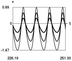
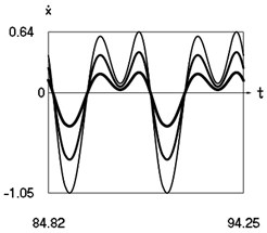
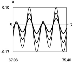
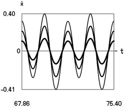
graphical relationships are obtained $x = x (t),$ $\dot{x} = \dot{x} (t),$ $\ddot{x} = \ddot{x} (t),$ $\dot{x} \ddot{x} = \dot{x} \ddot{x} (t),$ $\dot{x} = \dot{x} (x),$ $\ddot{x} = \ddot{x} (\dot{x})$ , $\dot{x} \ddot{x} = \dot{x} \ddot{x} (x)$ (see Fig. 1).

Fig. 1Dynamics of the system for the initial conditions of motion t=0, x0=0, x˙0= –1 (thin line), t=0, x0=0, x˙0= –2/3 (line of medium thickness) and t=0, x0=0, x˙0= –1/3 (thick line)

Dynamics of the system for the initial conditions of motion t=0, x0=0, x˙0= –1 (thin line), t=0, x0=0, x˙0= –2/3 (line of medium thickness) and t=0, x0=0, x˙0= –1/3 (thick line)

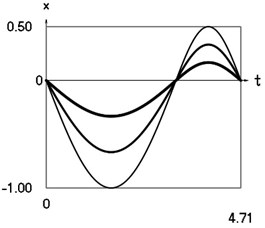
a) Displacement as function of time

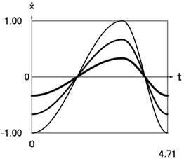
b) Velocity as function of time

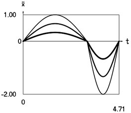
c) Acceleration as function of time

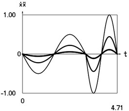
d) Velocity multiplied by acceleration as function of time

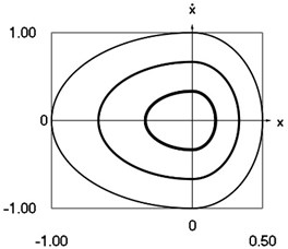
e) Phase trajectory: velocity as function of displacement

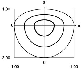
f) Phase trajectory: acceleration as function of velocity

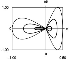
g) Phase trajectory: velocity multiplied by acceleration as function of displacement

According to the Eq. (12) eigenfrequency of the system:

20

\bar{ω} = 2 \frac{1 \cdot 2}{1 + 2} = \frac{4}{3} .

In the expansions into the Fourier series the first four members $n = 0,1, 2,3$ are taken into account.

By taking into account the Eqs. (11), (12) Table 1 is obtained.

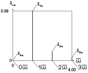
According to the Eqs. (13)-(17) by taking into account Eqs. (18)-(20) graphical relationships are obtained (see Fig. 2).

Table 1Analysis of harmonics

$n$	0	1	2	3	…	$n$
$n \bar{ω}$	0	$\frac{4}{3}$	$2 \cdot \frac{4}{3}$	$3 \cdot \frac{4}{3}$	…	$n \cdot \frac{4}{3}$
${\bar{T}}_{n} = \frac{2 π}{n \bar{ω}}$	$\infty$	$\frac{3}{2} π$	$\frac{3}{2 \cdot 2} π$	$\frac{3}{3 \cdot 2} π$	…	$\frac{3}{n \cdot 2} π$

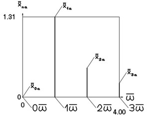
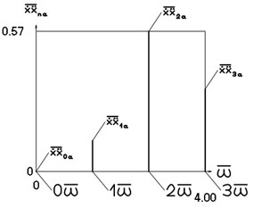
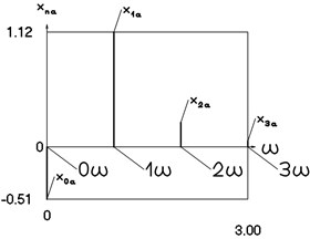
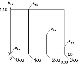
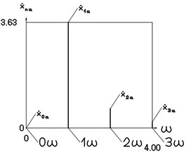
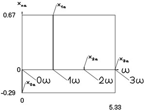
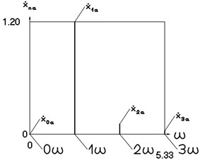
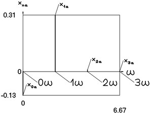
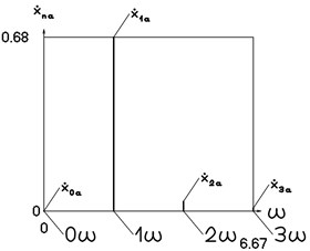
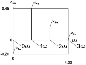
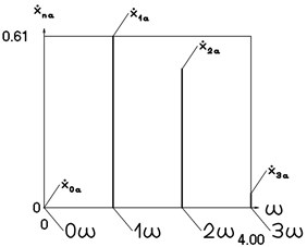
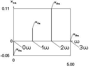
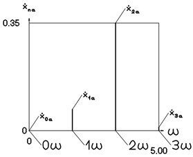
Fig. 2Amplitude frequency characteristics (constant part and first three harmonics)

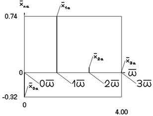
a) Displacement frequency characteristic

b) Velocity frequency characteristic

c) Acceleration frequency characteristic

d) Velocity multiplied by acceleration frequency characteristic

3. Forced vibrations

According to the Eqs. (1), (2) by assuming:

21

p_{1} = 1, p_{2} = 2, h_{1} = 0.1, h_{2} = 0.2, f \equiv v a r,

and at:

22

ω = \frac{3}{4} \bar{ω}, \bar{ω}, \frac{4}{3} \bar{ω}, \frac{5}{3} \bar{ω}, 2 \bar{ω}, \frac{5}{2} \bar{ω},

steady state solutions are found and their spectral analysis $ω$ , $2 ω$ , $3 ω$ , $4 ω$ , ... is performed.

Steady state solutions are presented in Fig. 3, Fig. 4, Fig. 5, Fig. 6, Fig. 7, Fig. 8.

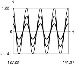
Fig. 3Steady state motions of the system for the first value of frequency of excitation and f= –1 (thin line), f= –2/3 (line of medium thickness), f= –1/3 (thick line)

Steady state motions of the system for the first value of frequency of excitation and f= –1 (thin line), f= –2/3 (line of medium thickness), f= –1/3 (thick line)

a) Displacement as function of time

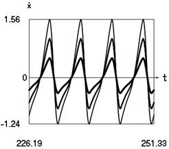
b) Velocity as function of time

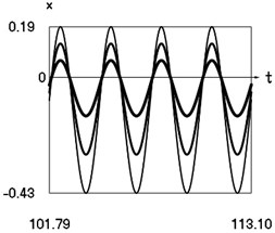
Fig. 4Steady state motions of the system for the second value of frequency of excitation and f= –1 (thin line), f= –2/3 (line of medium thickness), f= –1/3 (thick line)

Steady state motions of the system for the second value of frequency of excitation and f= –1 (thin line), f= –2/3 (line of medium thickness), f= –1/3 (thick line)

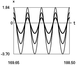
a) Displacement as function of time

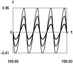
b) Velocity as function of time

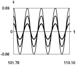
Fig. 5Steady state motions of the system for the third value of frequency of excitation and f= –1 (thin line), f= –2/3 (line of medium thickness), f= –1/3 (thick line)

Steady state motions of the system for the third value of frequency of excitation and f= –1 (thin line), f= –2/3 (line of medium thickness), f= –1/3 (thick line)

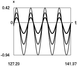
a) Displacement as function of time

b) Velocity as function of time

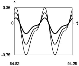
Fig. 6Steady state motions of the system for the fourth value of frequency of excitation and f= –1 (thin line), f= –2/3 (line of medium thickness), f= –1/3 (thick line)

Steady state motions of the system for the fourth value of frequency of excitation and f= –1 (thin line), f= –2/3 (line of medium thickness), f= –1/3 (thick line)

a) Displacement as function of time

b) Velocity as function of time

Fig. 7Steady state motions of the system for the fifth value of frequency of excitation and f= –1 (thin line), f= –2/3 (line of medium thickness), f= –1/3 (thick line)

Steady state motions of the system for the fifth value of frequency of excitation and f= –1 (thin line), f= –2/3 (line of medium thickness), f= –1/3 (thick line)

a) Displacement as function of time

b) Velocity as function of time

Fig. 8Steady state motions of the system for the sixth value of frequency of excitation and f= –1 (thin line), f= –2/3 (line of medium thickness), f= –1/3 (thick line)

Steady state motions of the system for the sixth value of frequency of excitation and f= –1 (thin line), f= –2/3 (line of medium thickness), f= –1/3 (thick line)

a) Displacement as function of time

b) Velocity as function of time

Amplitude frequency characteristics are presented in Fig. 9, Fig. 10, Fig. 11, Fig. 12, Fig. 13, Fig. 14.

Fig. 9Amplitude frequency characteristics (constant part and first three harmonics) for the first value of frequency of excitation

a) Displacement frequency characteristic

b) Velocity frequency characteristic

Fig. 10Amplitude frequency characteristics (constant part and first three harmonics) for the second value of frequency of excitation

a) Displacement frequency characteristic

b) Velocity frequency characteristic

Fig. 11Amplitude frequency characteristics (constant part and first three harmonics) for the third value of frequency of excitation

a) Displacement frequency characteristic

b) Velocity frequency characteristic

Fig. 12Amplitude frequency characteristics (constant part and first three harmonics) for the fourth value of frequency of excitation

a) Displacement frequency characteristic

b) Velocity frequency characteristic

Fig. 13Amplitude frequency characteristics (constant part and first three harmonics) for the fifth value of frequency of excitation

a) Displacement frequency characteristic

b) Velocity frequency characteristic

Fig. 14Amplitude frequency characteristics (constant part and first three harmonics) for the sixth value of frequency of excitation

a) Displacement frequency characteristic

b) Velocity frequency characteristic

4. Conclusions

On the basis of the presented results the qualities of dynamic behavior of the nonlinear vibrating system which consists from a mass between two linear elastic connecting members with different coefficients of stiffness can be used in different engineering applications requiring the stability in a wide range of parameters.

The motions of the system and amplitude frequency characteristics are determined by analytical – numerical method relationships. It is determined that for the case of the conservative system eigenfrequencies do not depend on the value of the amplitude of excitation. It is shown that for the case of forced harmonic excitation stable and unstable multivalued regimes do not exist in the system. Also, separate classes of nonlinear dynamical systems are investigated which have qualities of similar type.

The presented results enable to perform the design of nonlinear vibrating systems of this type. This enables to create new systems which can be noted by high stability properties, because in the vicinities of resonances they do not have multivalued solutions.

References

Bolotin V. V. Vibrations in Engineering. Handbook, Vol. 1, Mashinostroienie, Moscow, 1978, (in Russian).

Search CrossRef
Zaitsev V. A. Global asymptotic stabilization of periodic nonlinear systems with stable free dynamics. Systems and Control Letters, Vol. 91, 2016, p. 7-13.

Publisher
Salahshoor E., Ebrahimi S., Zhang Y. Frequency analysis of a typical planar flexible multibody system with joint clearances. Mechanism and Machine Theory, Vol. 126, 2018, p. 429-456.

Publisher
Starossek U. Forced response of low-frequency pendulum mechanism. Mechanism and Machine Theory, Vol. 99, 2016, p. 207-216.

Publisher
Wang S., Hua L., Yang C., Zhang Y., Tan X. Nonlinear vibrations of a piecewise-linear quarter-car truck model by incremental harmonic balance method. Nonlinear Dynamics, Vol. 92, 2018, p. 1719-1732.

Publisher
Alevras P., Theodossiades S., Rahnejat H. On the dynamics of a nonlinear energy harvester with multiple resonant zones. Nonlinear Dynamics, Vol. 92, 2018, p. 1271-1286.

Publisher
Sinha A., Bharti S. K., Samantaray A. K., Chakraborty G., Bhattacharyya R. Sommerfeld effect in an oscillator with a reciprocating mass. Nonlinear Dynamics, Vol. 93, 2018, p. 1719-1739.

Publisher
Habib G., Cirillo G. I., Kerschen G. Isolated resonances and nonlinear damping. Nonlinear Dynamics, Vol. 93, 2018, p. 979-994.

Publisher
Ragulskis K., Bansevičius R., Barauskas R., Kulvietis G. Vibromotors for Precision Microrobots. Hemisphere, New York, 1987.

Search CrossRef

About this article

Received

15 July 2019

Accepted

20 August 2019

Published

30 September 2019

DOI

https://doi.org/10.21595/mme.2019.20942

Keywords

nonlinear system

coefficients of stiffness

amplitude-frequency characteristics

dynamical qualities

This is an open access article distributed under the Creative Commons Attribution License, which permits unrestricted use, distribution, and reproduction in any medium, provided the original work is properly cited.

Previous article in issue Previous Next article in issue Next

Research article

2022 08 15

Assessing the nonlinear static stiffness of rail pad using finite element method

Muhammad Iqbal Haikal Othman, Abdul Malek Abdul Wahab, Muhamad Sukri Hadi, Noraishah Mohamad Noor

Research article

2018 02 15

Dynamical response of fractional-order nonlinear system with combined parametric and forcing excitation

Hai Jun Xing, Ke Shi Xiao, Peng Sai Song, Lin Ru Li

Research article

2017 02 15

Stability and nonlinear self-excited friction-induced vibrations for a minimal model subjected to multiple coalescence patterns

Mzaki Dakel, Jean-Jacques Sinou

Research article

2016 12 31

Analytical model for nonlinear vibration of flexible rotor system

Min Wu, Shengbo Yang, Dongjiang Han, Daren Yu, Jinfu Yang

K. Ragulskis and L. Ragulskis, “Vibrations of the nonlinear system in which stationary harmonic excited multivalued regimes in the vicinities of resonances do not exist,” Mathematical Models in Engineering, Vol. 5, No. 3, pp. 97–104, Sep. 2019, https://doi.org/10.21595/mme.2019.20942

Copy Extrica

Copied to clipboard!

TY  - JOUR
DO  - 10.21595/mme.2019.20942
UR  - https://doi.org/10.21595/mme.2019.20942
TI  - Vibrations of the nonlinear system in which stationary harmonic excited multivalued regimes in the vicinities of resonances do not exist
T2  - Mathematical Models in Engineering
AU  - Ragulskis, K.
AU  - Ragulskis, L.
PY  - 2019
DA  - 2019/09/30
PB  - JVE International Ltd.
SP  - 97-104
IS  - 3
VL  - 5
SN  - 2351-5279
SN  - 2424-4627
ER  - 

Copy Ris

Copied to clipboard!

@article{Ragulskis_2019,
	doi = {10.21595/mme.2019.20942},
	url = {https://doi.org/10.21595/mme.2019.20942},
	year = 2019,
	month = {sep},
	publisher = {{JVE} International Ltd.},
	volume = {5},
	number = {3},
	pages = {97--104},
	author = {K. Ragulskis and L. Ragulskis},
	title = {Vibrations of the nonlinear system in which stationary harmonic excited multivalued regimes in the vicinities of resonances do not exist},
	journal = {Mathematical Models in Engineering}
}

Copy Bibtex

Copied to clipboard!

[1]K. Ragulskis and L. Ragulskis, “Vibrations of the nonlinear system in which stationary harmonic excited multivalued regimes in the vicinities of resonances do not exist,” Mathematical Models in Engineering, vol. 5, no. 3, pp. 97–104, Sep. 2019, doi: 10.21595/mme.2019.20942.

Copy IEEE

Copied to clipboard!

Ragulskis, K., and L. Ragulskis. “Vibrations of the Nonlinear System in Which Stationary Harmonic Excited Multivalued Regimes in the Vicinities of Resonances Do Not Exist.” Mathematical Models in Engineering 5, no. 3 (September 30, 2019): 97–104. https://doi.org/10.21595/mme.2019.20942.

Copy Chicago

Copied to clipboard!

Vibrations of the nonlinear system in which stationary harmonic excited multivalued regimes in the vicinities of resonances do not exist

Abstract

1. Introduction

2. The conservative system

3. Forced vibrations

4. Conclusions

References

About this article

Related Articles