Abstract
Compressive sensing provides a new idea for machinery monitoring, which greatly reduces the burden on data transmission. After that, the compressed signal will be used for fault diagnosis by feature extraction and fault classification. However, traditional fault diagnosis heavily depends on the prior knowledge and requires a signal reconstruction which will cost great time consumption. For this problem, a deep belief network (DBN) is used here for fault detection directly on compressed signal. This is the first time DBN is combined with the compressive sensing. The PCA analysis shows that DBN has successfully separated different features. The DBN method which is tested on compressed gearbox signal, achieves 92.5 % accuracy for 25 % compressed signal. We compare the DBN on both compressed and reconstructed signal, and find that the DBN using compressed signal not only achieves better accuracies, but also costs less time when compression ratio is less than 0.35. Moreover, the results have been compared with other classification methods.
1. Introduction
The monitoring of machinery is becoming increasingly important in the manufacturing field today. With progress of mechanical technology, the machinery tends to be large, complex, and functional. Once facing failure, it will cause abnormal event progression and huge productivity loss. For this consideration, a great number of operating data are required to evaluate the machinery states in real time. However, such monitoring will put tremendous burden on data transmission and storage. There is a lot of data redundant which leads to huge waste of resources, as well. The compressive sensing (CS) [1-3] theory provides a new idea in solving this problem. The CS enables the recovery of a sparse signal from a few of its measurements. The amount of data collected under CS framework is much smaller, which achieves a breakthrough of Nyquist sampling theory. Thus, it has been widely used in the photography and data processing fields.
Fault diagnosis is the key to the prognostic and health management (PHM). And typical fault diagnosis methods contain two steps: feature extraction and fault classification with a classifier. For vibration signals, there are time-domain [4] and frequency-domain [5] techniques for feature extraction. Time-domain feature extraction techniques can be further categorized into three groups: statistical-based [6], model-based [7], and signal processing –based [8] approaches. Time-domain features are considered to be good for fault diagnosis, but less effective for fault classification, while frequency-domain features are more effective for fault classification. Typical methods include spectral analysis, envelope analysis, cepstrum, et al. Then, clustering algorithms [9], dimension reduction algorithms [10], support vector machine (SVM) [11], and neural network [12, 13] are normally used to achieve fault classification. Moreover, some time-frequency-domain methods also merge in recent years. These methods include empirical mode decomposition (EMD) [14], wavelet transform (WT) [15] and so on.
However, there are still some disadvantages for traditional fault diagnosis. For example, the feature extraction is usually conducted based on the prior knowledge of people. The performance of fault diagnosis largely depends on selected signal processing and appropriate feature extraction. Once the features are not sensitive to the faults, the classification will be hard to achieve. Moreover, a large amount of training is required before recognition.
For the past few years, a few researchers have been studying the use of CS in machinery monitoring and fault diagnosis. Zhou [16] proposed a new feature extraction method based on CS theory. They compare the original feature vectors and real-time features to identify the fault. The new diagnosis algorithm is validated for an induction motor. Du [17] performed the feature-identification directly on compressed signal, and they proposed an alternating direction method for CS problem solving. Sun [18] proposed a compressed data reconstruction scheme for signal acquisition and bearing monitoring. The block sparse Bayesian learning method utilizes the block property and presents great capability of signal recovering. Tang [19] studied extract fault features using down-sampling method. The MP algorithm has been used for incomplete reconstruction of the specific harmonic components.
Deep learning [20] methods have developed rapidly in the field of fault diagnosis in recent years. As one of the classical deep learning models, a deep belief network (DBN) [21] overcomes the disadvantages of traditional methods with its special structure. The DBN model has powerful automatic feature extraction capability. It can obtain low-dimensional features from the high-dimensional complex signals efficiently, thus enhancing the intelligence of the fault diagnosis process [22]. Early DBN is mainly used for speech signal recognition [23], image processing, and some other areas. However, increasing scholars have applied DBN into the fault diagnosis field. Dan [24] et al studied DBN for identifying the bearing failure, and compared it with support vector machine (SVM), back propagation neural network (BPNN). Pan [25] et al proposed a new approach for high-voltage circuit breaker mechanical fault diagnosis. The DBN model was used for deep mining and adaptive feature extraction, combined with transfer learning method to improve classification accuracy. Chen [26] et al proposed a DBN-based DNN model for gearbox fault detection. They used load, speed, time-domain, and frequency-domain features as model input, and achieved good classification results. For better effects, Tao [27] et al collected multiple vibration signals as training samples. Then they utilized the learning ability of DBN to adaptively fuse the multi-feature data. The experimental results showed that DBN models obtained higher classification accuracy than SVM, BPNN, and KNN.
Machinery health monitoring is entering the Big Data era and places more demands on machine health monitoring. There is a huge need for data compression that can decrease the burden of data storage and transmission. For this purpose, compressive sensing and DBN have been merged, forming a new machinery health monitoring system. This paper combines the DBN model and compressive sensing for fault diagnosis. First, we acquire the projections of the original signal according to CS theory. Then, we consider achieving fault diagnosis using CS compressed signal directly, because the main information is reserved in the measurements. The DBN model is selected since it achieves feature extraction automatically. The DBN can learn the features from a complex compressed signal adaptively and incorporate nonlinear relationships between machinery states and compressed signals.
The contributions of this paper are decomposed into two aspects: (1) we detect the machinery faults using CS compressed signal instead of original or reconstructed signal. This approach can avoid the complex reconstruction process and save computing resources. (2) The DBN model is introduced here for its strong capability of feature extraction and fault diagnosis.
2. Related work: compressive sensing and deep belief network
2.1. Compressive sensing
In the framework of CS, a measurement matrix has been designed for reducing the dimension of original signal . Each row of the measurement matrix can be seen as a filter for obtaining linear projections. And parts of the signal information can be obtained by each filter. In summary, the compressive projections can be represented as:
Then, a low-dimensional signal is used to present the high-dimensional signal . Generally, we can not directly recover the original signal from measurement when . However, if is sparse, this recovery can be achieved since more information is known.
In the CS theory, a sparse basis is needed for decomposition. If we decompose original signal on the sparse basis, then vector can be represented as:
where can be seen as the sparse coefficients. Eq. (2) is equivalent to:
where and . Here, is defined as a column vector. Combining Eqs. (1) and (3), we can represent signal as:
where is defined as sensing matrix. Solving a sparse vector is a commonly discussed problem [2, 28] with respect to . The framework of CS is shown in Fig. 1.
According to Candès and Tao, for higher successfully probability of recovery, the sensing matrix must follow the restricted isometry property (RIP), that is:
where represents a random -sparse vector, and (0, 1). After sparse vector being obtained, the original signal is easily achieved using Eq. (3).
Fig. 1The framework of compressive sensing

2.2. The basic units of DBN
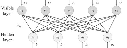
DBN is consist of multiple restricted Boltzmann machines (RBM) and classifiers. RBM is the basic unit of DBN, which comprises two layers of neural network: visible layer and hidden layer. The visible layer and hidden layer are connected through weight and biases vectors , . However, the units in same layer are not connected, respectively. The structure of RBM is shown as Fig. 2.
For given visible layer and hidden layer , the energy function can be represented as:
where , represent the binary states of units, , represent the node biases, and represents the weight. The main purpose of DBN model is to find a stable state, which minimizes the energy error. Therefore, joint probability distribution between visible layer and hidden layer can be represented as follow:
where is the energy summary of all visible and hidden layers. Eq. (7) can be seen as a proportional function for guaranteeing the normalized distribution. Moreover, the probability distributions of visible and hidden vectors can be calculated by:
Eq. (9) represents the learning process, that is to extract low-dimensional features from high-dimensional input data. And Eq. (10) represents a reverse learning process in which input data is reconstructed from feature vectors.
Fig. 2The structure of RBM
2.3. The DBN training
The DBN training consists of two steps: (1) For RBM units, a pre-training is performed between two layers using unlabeled data. (2) The fine-tuning is performed utilizing the backpropagation algorithm to adjust the parameters. The first step is an unsupervised learning process, while the second is a supervised process.
Fig. 3The pre-training process of DBN
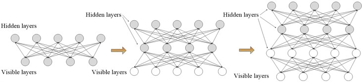
The pre-training process is shown in Fig. 3, and the dark layer represents the training part for each step. In the pre-training process, a stochastic gradient descent on the negative log-likelihood probability is used for training RBM. The function is defined as follow:
where denotes the data expectation of distribution, and denotes the model expectation of distribution. In the actual application, obtaining the precise value of is so difficult. Thus, it is substituted by iterations of Gibbs sampling as the final results. The parameters are updated as follow:
where denotes the input sample. From Eq. (12), the data generated by a visible layer is passed to the hidden layer. And then the hidden layer is used to reconstruct that vector. During this process, all parameters , , of DBN will be updated until the number of iterations is satisfied.
After pre-training, the next step is fine-tuning. The ultimate purpose of this step is to further decrease the training error and improve the classification accuracy. Generally, a backpropagation neural network (BPNN) algorithm is performed to adjust the parameters. Assume that the label of input is , and the output of DBN is , with training error as defined below:
where represents the error parameter. With the advancement of iterations, will be updated as follow:
where denotes the learning ratio. The supervised training will continue until the error is less than a certain setting.
3. DBN for CS compressed signal
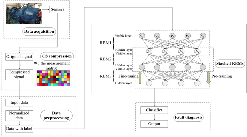
This paper introduces the DBN model to fault diagnosis of CS compressed signal. The framework of proposed method can be seen as Fig. 4. Compared to traditional fault diagnosis model, the benefits of this article include:
(1) The approach greatly improves the efficiency of health monitoring, and saves the processing time of the management node. Generally, an accurate reconstruction algorithm means more running time. Referring [29], the Lap-CBCS-KSVD algorithm can be seen as one of the most accurate algorithms. However, it costs much more time than traditional basic pursuit (BP), orthogonal matching pursuit (OMP) algorithms. In this paper, we abandon the step of reconstruction and directly perform fault diagnosis on compressed signal, thus avoiding a lot of computation time.
(2) This paper fully utilizes the automatic feature extraction capability of DBN. Since the compressed signal changes original timing relationship, it is meaningless to perform feature extraction with traditional methods, such as time-domain analysis and frequency-domain analysis. However, the strong feature extraction capabilities of DBN make it possible to obtain the information preserved in compressed signal.
Table 1Flow chart of this approach
Step | Description |
Step 1 (data acquisition) | Collect raw data from the machinery |
Step 2 (CS compression) | Compress the original signal with measurement matrix according to CS theory |
Step 3 (data preprocessing) | Normalize the input data and make label for each training sample |
Step 4 (stack RBMs) | Stack multiple RBMs layer by layer, then perform pre-training and fine-tuning to adjust the RBM weights and offsets |
Step 5 (fault diagnosis) | A classifier is accessed to the top of RBM, and the samples are classified to corresponding categories |
In this paper, we apply the DBN model to adaptively extract features from compressed signal and perform fault classification based on these features. There are five main processes in proposed method: data acquisition, CS compression, data preprocessing, stack RBMs, and fault diagnosis. Table 1 summarizes the procedure of this approach. As shown in Fig. 4, the CS compression uses a preset measurement matrix to perform dimensional reduction projection on the original signal. Before DBN training, the compressed data is first normalized and assigned a label. The DBN model consists of several stacked RBMs, which is used for DBN training. The training process can be divided into two steps: pre-training and fine-tuning. More details about these two steps have been illustrated in section 2.3. Then, a classifier is linked to the RBM output, and the testing samples can be classified to the corresponding fault type according to the label. From above discussion, the innovation of this paper refers to the implementation elements, and we must acknowledge that there are few improvements to the initial DBN model.
Fig. 4DBN model for compressed signal diagnosis
4. Experiment
4.1. DBN fault diagnosis on compressed gearbox signals
In order to measure the validity of DBN-CS approach, a gearbox experimental platform is set up as in Fig. 5. The experimental table is constituted with motor, torque decoder and power tester. The experiments are conducted under following speeds, 400 rpm, 800 rpm and 1200 rpm. For each speed, four kinds of loads are applied using magnetic powder brake and they are 0 Nm, 0.4 Nm, 0.8 Nm, and 1.2 Nm.
Fig. 5Planetary gearbox test rig
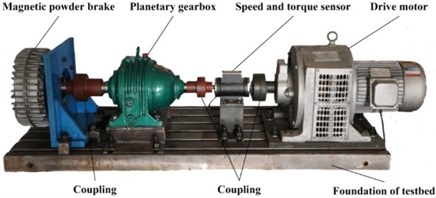
Fig. 6Seeded wear failure
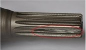
a) Sun gear

b) Planet gear
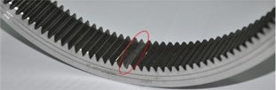
c) Ring gear
Table 2Training and testing samples
State of signal | Load (Nm) | Speed (rpm) | Number of training samples | Number of testing samples |
Normal state | 0 | 400 | 150 | 50 |
0.4 | 800 | 150 | 50 | |
0.8 | 1200 | 150 | 50 | |
Planet gear failure | 0 | 400 | 150 | 50 |
0.4 | 800 | 150 | 50 | |
0.8 | 1200 | 150 | 50 | |
Ring gear failure | 0 | 400 | 150 | 50 |
0.4 | 800 | 150 | 50 | |
0.8 | 1200 | 150 | 50 | |
Sun gear failure | 0 | 400 | 150 | 50 |
0.4 | 800 | 150 | 50 | |
0.8 | 1200 | 150 | 50 |
For methods testing, four conditions are applied to the system. One of them is the normal state to compare with three faulty states: sun gear fault, planet gear fault, and ring gear fault. The specific failures are shown in Fig. 6. The sampling frequency is set to 20 kHz and acquired vibration signal has a 12 s duration for each sample. The training and testing samples are listed in Table 2. It can be seen that the number of training samples for each state is 450, and that of testing samples is 150. We will calculate the success accuracies for both training samples and testing samples in the experiments.
In compressive sensing, the compression ratio (CR) is often analyzed for evaluating the compression. Assuming that the length of original signal is and the length of compressed signal is , then we have:
We firstly take the 25 % compressed signal ( 25 %) for example to validate the proposed method. The measurement matrix is designed using the Toeplitz matrix with Gaussian entries as the basis. In this way, the Toeplitz matrix generated by Gaussian entries is supposed to achieve higher reconstruction accuracies. Since 25 %, the dimension of measurement matrix should be set as (0.75 ).
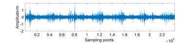
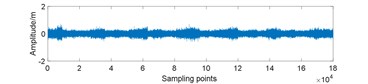
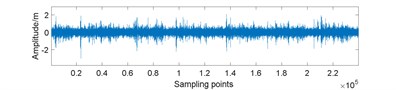
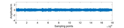
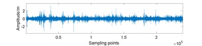
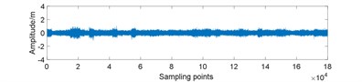
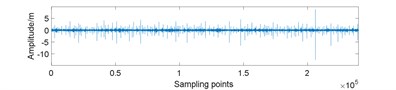
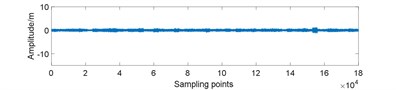
Fig. 7Amplitudes waveform of original and 25 % compressed signal for gearbox in different conditions: a) normal; b) normal and compressed; c) planet gear fault; d) planet gear fault and compressed; e) ring gear fault; f) ring gear fault and compressed; g) sun gear fault; h) sun gear fault and compressed
a)
b)
c)
d)
e)
f)
g)
h)
In the data preparation phase, we split the entire signal into small samples because the raw signal is too long. It is impossible to perform such high-dimensional matrix operation. Then, we put the compressed signal samples together to reunion the entire compressed signal. As Fig. 7 displays, the peak value of compressed signal is lower and the signal fluctuation is smaller compared to original signal.
Table 3The configurations of DBN model
Parameters | Value |
Initial learning rate | 0.01 |
Initial momentum | 0.5 |
Sample length | 3000 |
Numepochs | 100 |
Batchsize | 100 |
Method | CD |
The experimental environment is set as follow: the computer processor is Intel(R) Core(TM) i5-8250U 1.6 GHz, and the simulation tool is Matlab R2017a. Moreover, there are some important parameters of DBN requiring careful choices, for example the sample length. Because the number of sampling points in one cycle is 3000, we set the sample length as 4000. And the compressed signal length is 4000×75 % = 3000. The fine-tuning process utilizes BP algorithm to distribute errors of two RBM. The momentum and the learning rate are two factors describing weight updating criteria between two RBM layers. Moreover, a Contrast Divergence (CD) algorithm is used for obtaining the expected value of the energy partial derivative function [30]. The related parameters of DBN are shown in Table 3.
The structure of DBN is another important factor that affects the diagnosis accuracy. For example, structure 3000-600-600-4 means the input layer includes 3000 nodes, and the output layer includes 4 nodes. Since the input and output nodes are certain, we abbreviate the structure as 600-600. Table 4 displays the experimental results of different DBN structures.
Table 4The DBN fault diagnosis results of 25 % compressed signal for different structures
Hidden layer nodes | Accuracy of training samples | Accuracy of testing samples | Training time / s |
200-200 | 63.5 % | 47.5 % | 151.88 |
300-300 | 95.2 % | 72.5 % | 175.99 |
400-400 | 100 % | 80 % | 180.53 |
500-500 | 100 % | 85 % | 202.69 |
600-600 | 100 % | 92.5 % | 228.47 |
700-700 | 100 % | 90 % | 246.68 |
800-800 | 100 % | 87.5 % | 268.88 |
800-200-50 | 60 % | 40 % | 279.44 |
800-300-100-50 | 33.5 % | 30 % | 293.81 |
It can be seen from the Table 4 that the structure 600-600 achieves the best accuracy 95 %, and average training time is 228.47 s. We can also find that more layers do not mean higher accuracies and two layers is the most efficient.
Fig. 8The confusion matrix of DBN classification
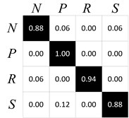
Fig. 9PCA analysis of the DBN learned features
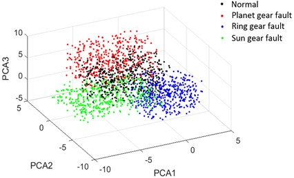
The confusion matrix of best result for DBN diagnosis is shown in Fig. 8. It is observed that the planet gear fault (P) has the best accuracy of 100 %, ring gear fault (R) has the accuracy of 94 %, and normal state (N), sun gear fault (S) have the worst accuracy of 88 %. To gain more insight about the capability of DBN, a principal component analysis (PCA) method is used to show the separability of extracted features. The features obtained from the 1st layer of DBN have been decreased to 3 kinds: PCA1, PCA2, PCA3 as Fig. 9 shows.
More experiments have been conducted for different compressed signals. Table 5-7 display the DBN fault diagnosis results of 10 %, 20 % and 40 % compressed signals. In the testing experiments, DBN achieves 95.17 % identification accuracy for 10 % compressed signal, 92.9 % identification accuracy for 20 % compressed signal, and 64.5 % identification accuracy for 40 % compressed signal. The average training time for appeal results are 265.85 s, 257.14 s, and 196.47 s. With the compression ratio increasing, the accuracies of training samples and testing samples fall down because the useful features have been destroyed gradually.
Table 5The DBN fault diagnosis results of 10 % compressed signal for different structures
Hidden layer nodes | Accuracy of training samples | Accuracy of testing samples | Training time / s |
100-100 | 92.5 % | 87.3 % | 205.59 |
200-200 | 100 % | 93 % | 238.29 |
300-300 | 100 % | 95.17 % | 265.85 |
400-400 | 100 % | 94 % | 275.12 |
500-500 | 100 % | 92 % | 296.77 |
600-600 | 93.1 % | 87.3 % | 303.48 |
700-700 | 91.2 % | 88.5 % | 324.74 |
800-800 | 87.5 % | 85 % | 349.07 |
900-900 | 90 % | 88.5 % | 362.09 |
Table 6The DBN fault diagnosis results of 20 % compressed signal for different structures
Hidden layer nodes | Accuracy of training samples | Accuracy of testing samples | Training time / s |
500-500 | 89.7 % | 85.8 % | 217.80 |
600-600 | 99.2 % | 90.1 % | 222.26 |
700-700 | 100 % | 91.9 % | 234.73 |
800-800 | 80.5 % | 79.4 % | 248.15 |
900-900 | 97.5 % | 88.3 % | 242.30 |
1000-1000 | 100 % | 92.9 % | 257.14 |
1100-1100 | 95 % | 86.5 % | 267.69 |
1200-1200 | 83.2 % | 79.4 % | 272.41 |
Table 7The DBN fault diagnosis results of 40 % compressed signal for different structures
Hidden layer nodes | Accuracy of training samples | Accuracy of testing samples | Training time / s |
100-100 | 63.7 % | 61.3 % | 186.81 |
200-200 | 63.5 % | 61.3 % | 190.38 |
300-300 | 52.6 % | 51.9 % | 192.7 |
400-400 | 67 % | 64.5 % | 196.47 |
500-500 | 52.2 % | 51.9 % | 199.8 |
600-600 | 58.8 % | 58.2 % | 202.89 |
700-700 | 43.1 % | 42.5 % | 207.13 |
800-800 | 55.6 % | 55 % | 210.45 |
900-900 | 52.4 % | 51.9 % | 213.76 |
4.2. Comparison with other classification methods
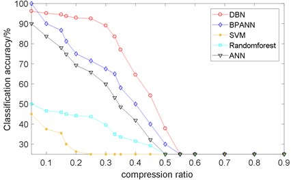
In order to verify the validation of proposed method, the comparative fault diagnosis methods are tested, such as BP artificial neural network (BPANN), support vector machine (SVM), random forest (RF), and artificial neural network (ANN). The structure of BPANN and ANN is 3000-600-100-4, indicating that there are two layers between input and output. The penalty factor and the radius for SVM classifier is set as 0.216 and 0.3027, referring [27]. The compression ratio varies from 0.05 to 0.9. The algorithms of BPANN, SVM, RF, ANN and DBN trained the model with the same compressed data set and generated a classifier to perform the classification. For each data point, 100 experiments have been performed. And we calculate the average value to evaluate different methods as Fig. 10 shows.
It is inferred that the DBN model is better for compressed signal fault diagnosis, especially when CR is 0.1-0.3. We can also find that BPANN achieves 100 % accuracy when 0.05, which is better than DBN. This is because the main features have been reserved in the compressed signal when CR is low, and BPANN extracts them efficiently. However, as the compression ratio increases, the information of original signal loses gradually. At this time, DBN achieves better performance for its strong feature extraction capability.
Fig. 10Comparison of different classification methods
4.3. Comparison of compressed and reconstructed signal
Here, a comparison of DBN diagnosis on compressed signal and reconstructed signal has been proposed. In traditional monitoring, the compressed signal is firstly reconstructed and then used for diagnosis. However, this may cause great time consumption because of the complex reconstruction algorithms. Therefore, we try to replace this process with DBN diagnosis directly on compressed signal. The new framework is shown in Fig. 11.
In order to compare those two approaches, a Bayesian compressive sensing algorithm is used here for signal reconstruction. For CS theory, the reconstruction algorithms can be divided into three categories: greedy-based methods, convex optimization methods [28], and Bayesian compressive sensing methods [31]. The Bayesian method estimates the maximum posterior probability from a Bayesian perspective. The Bayesian methods are more accurate than the other two kinds, in spite of a bigger time cost.
Referring Section 2, the key to compressive sensing is obtaining a strong sparse representation of original signal . Extended by -means clustering, K-SVD algorithm [32] adaptively produces the sparse dictionary by training signal blocks. Compared to fixed dictionaries, such as discrete cosine transform, Fourier transform, K-SVD algorithm avoids the dependence on prior knowledge.
Fig. 11The new diagnosis framework based on DBN method
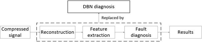
Fig. 12 displays the DBN classification results on both compressed signal and reconstructed signal. The compression ratio (CR) varies from 0.1 to 0.6. With CR increasing, the accuracy of compressed signal falls down quickly, while the accuracy of reconstructed signal is relatively stable. Moreover, it can be seen that the accuracies of compressed signal are superior to those of reconstructed signal when CR varies from 0.1-0.35. In this stage, there is sufficient information preserved in compressed signal for DBN diagnosis. When CR is larger than 0.35, the features in compressed signal are destroyed seriously, which leads to a poor accuracy. At this time, the precisely reconstructed signal presents great potential for DBN diagnosis.
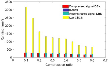
Similarly, Fig. 13 indicates the comparison of running time on both compressed signal and reconstructed signal. The running time of reconstructed signal includes three parts: K-SVD training, Lap-CBCS reconstruction, and the DBN diagnosis. It is found that the DBN running time of compressed signal and reconstructed signal is not much different. However, the total running time of reconstructed signal is far more than that of compressed signal.
Fig. 12The DBN classification accuracy of compressed signal and reconstructed signal
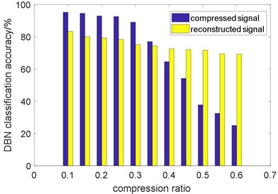
Fig. 13The running time of compressed signal and reconstructed signal
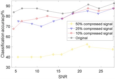
4.4. The effects of noise
In actual signal acquisition process, the noise generated by working machinery and sensor may have influences on data compression and fault diagnosis. To further study the influence of noise, the 10 % compressed, 25 % compressed, and 50 % compressed signals are chosen for comparison. Assuming that the noise follows Gaussian distribution, a random white noise is introduced after signal compression. The signal received is re-defined as:
where vector represents the noise signal. For evaluating the noisy level, the signal to noise (SNR) is denoted as:
As shown in Fig. 14, four curves demonstrate that the diagnostic accuracies increase gradually with the increasing SNR. And the 10 %, 25 % compressed signal are not much different with the original signal as SNR varies from 16 to 28.
In conclusion, it has little influence on compressed signals when noise is relatively small (16 28). This indicates a strong robustness of DBN diagnosis method on CS compressed signal. However, compared to the original signal, the compressed signals are kind of unstable with the SNR increasing.
Fig. 14The DBN classification accuracy of original and compressed signal for different SNR
5. Conclusions
Implementation of DBN diagnosis on compressed signal has been developed in this paper. This approach adaptively extracts the features preserved in compressed signal, and achieves fault diagnosis through stacked RBM learning. The main conclusions are obtained as follows:
1, For 10 %, 20 %, 25 % and 40 % compressed signal, the DBN approach achieves the accuracies of 95.17 %, 92.9 %, 92.5 %, 64.5 %, respectively.
2, The comparison of DBN with typical classification methods, such as BPANN, ANN, SVM, Random forest, has been conducted. It suggests that DBN is more effective for compressed signal diagnosis than other methods,
3, Another comparison of DBN on both compressed signal and reconstructed signal has been conducted as well. We have found that the DBN for compressed signal not only achieves better accuracies when CR is 0.1-0.35, but also cost much less time.
4, The effects of noise on compression and reconstruction have been studied as well. And we have found that it has little influence when noise is relatively small, which indicates the robustness of proposed method.
The limitations of DBN diagnosis include the following aspects. Firstly, there are a lot of parameters, such as learning rate, momentum, numepoch, batchsize, sample length, which may influence the results of fault diagnosis. A parameter optimization method is recommended for better classification performance. Moreover, the DBN method takes more time than classical classification methods, such as SVM, Random forest, BPANN. It can be modified to reduce the training time.
References
-
Candès E. J. Compressive sampling. Proceedings of International Congress of Mathematics, Madrid, Spain, Vol. 3, 2006, p. 1433-1452.
-
Candès E. J., Tao T. Decoding by linear programming. IEEE Transactions on Information Theory, Vol. 51, Issue 12, 2005, p. 4203-4215.
-
Donoho D. L. Compressed sensing. IEEE Transactions on Information Theory, Vol. 52, Issue 4, 2006, p. 1289-1306.
-
Tandon N., Choudhury A. A review of vibration and acoustic measurement methods for the detection of defects in rolling element bearings. Tribology International, Vol. 32, 1999, p. 469-480.
-
McFadden P. D., Smith J. D. Vibration monitoring of rolling element bearings by the high-frequency resonance technique – a review. Tribology International, Vol. 17, 1984, p. 3-10.
-
Heng R. B., Nor M. J. Statistical analysis of sound and vibration signals for monitoring rolling element bearing condition. Applied Acoustics, Vol. 53, 1998, p. 211-226.
-
Chu Q. Q., Xiao H., Lü Y., et al. Gear fault diagnosis based on multifractal theory and neural network. Journal of Vibration and Shock, Vol. 34, Issue 21, 2015, p. 15-18.
-
Luo Y., Zhen L. J. Diagnosis method of turbine gearbox gearcrack based on wavelet packet and cepstrum analysis. Journal of Vibration and Shock, Vol. 34, Issue 3, 2015, p. 210-214.
-
Zhao H. M., Zheng J. J., Xu J. J., Deng W. Fault diagnosis method based on principal component analysis and broad learning system. IEEE Access, Vol. 7, 2019, p. 99263-99272.
-
Goldberg D. E. Genetic Algorithms in Search, Optimization and Machine Learning. Addison Wesley Publishing Company Inc, New York, 1989.
-
Zhang C., Chen J. J., Guo X., et al. Gear fault diagnosis method based on ensemble empirical mode decomposition energy entropy and support vector machine. Journal of Central South University, Vol. 43, Issue 3, 2012, p. 932-939.
-
Ali J. B., Fnaiech N., Saidi L., et al. Application of empirical mode decomposition and artificial neural network for automatic bearing fault diagnosis based on vibration signals. Applied Acoustics, Vol. 89, Issue 3, 2015, p. 16-27.
-
Ke L., Peng C., Wang S. An intelligent diagnosis method for rotating machinery using least squares mapping and a fuzzy neural network. Sensors, Vol. 12, Issue 5, 2012, p. 5919-5939.
-
Zhao H. M., Sun M., Deng W., Yang X. H. A new feature extraction method based on EEMD and multi-scale fuzzy entropy for motor bearing. Entropy, Vol. 19, 2017, p. 14.
-
Wang S. B., Huang W. G., Zhu Z. K. Transient modeling and parameter identification based on wavelet and correlation filtering for rotating machine fault diagnosis. Mechanical Systems and Signal Processing, Vol. 25, 4, p. 1299-1320.
-
Zhou Z. H., Zhao J. W., Cao F. L. A novel approach for fault diagnosis of induction motor with invariant character vectors. Information Sciences, Vol. 281, 2014, p. 496-506.
-
Du Z. H., Chen X. F., Zhang H., Miao H. H., Guo Y. J., Yang B. Y. Feature identification with compressive measurements for machine fault diagnosis. IEEE Transactions on Instrumentation and Measurement, Vol. 65, 2016, p. 977-987.
-
Sun J. D., Yu Y., Wen J. T. Compressed-sensing reconstruction based on block sparse Bayesian learning in bearing-condition monitoring. Sensors, Vol. 17, 2017, p. 1454.
-
Tang G., Hou W., Wang H., Luo G., Ma J. Compressive sensing of roller bearing faults via harmonic detection from under-sampled vibration signals. Sensors, Vol. 15, 2015, p. 25648-25662.
-
Schmidhuber J. Deep learning in neural networks: an overview. Neural Networks, Vol. 61, 2015, p. 85-117.
-
Hinton G. E., Salakhutdinov R. R. Reducing the dimensionality of data with neural networks. Science, Vol. 313, Issue 5786, 2006, p. 504-507.
-
Zhang Q., Yang L. T., Chen Z. Deep computation model for unsupervised feature learning on big data. IEEE Transactions on Services Computing, Vol. 9, Issue 1, 2016, p. 161-171.
-
Hinton G., Deng L., Yu D., et al. Deep neural networks for acoustic modeling in speech recognition: The shared views of four research groups. IEEE Signal Processing Magazine, Vol. 29, Issue 6, 2012, p. 82-97.
-
Dan Q., Liu X., Chai Y., Zhang K., Li H. A fault diagnosis approach based on deep belief network and its application in bearing fault. Chinese Intelligent Systems Conference, Lecture Notes in Electrical Engineering, Vol. 528, 2018, p. 289-300.
-
Pan Y., Mei F., Miao H. Y., Zheng J. Y., Zhu K. D., Sha H. Y. An approach for HVCB mechanical fault diagnosis based on a deep belief network and a transfer learning strategy. Journal of Electrical Engineering and Technology, Vol. 14, 2019, p. 407-419.
-
Chen Z., Li C., Sánchez R. V. Multi-layer neural network with deep belief network for gearbox fault diagnosis. Journal of Vibroengineering, Vol. 17, Issue 5, 2015, p. 2379-2392.
-
Tao J., Liu Y. L., Yang D. L. Bearing fault diagnosis based on deep belief network and multisensor information fusion. Shock and Vibration, Vol. 2016, 2016, p. 9306205.
-
Tropp J. A. Computational methods for sparse solution of linear inverse problems. Proceedings of the IEEE Special Issue on Applications of Sparse Representation and Compressive Sensing, 2009.
-
Ma Y., Jia X., Hu Q., Xu D., et al. Laplace prior-based Bayesian compressive sensing using K-SVD for vibration signal transmission and fault detection. Electronics, Vol. 8, 2019, p. 517.
-
Shan W., Zeng X. Signal reconstruction and bearing fault recognition based on deep belief network. Journal of Engineering Design, Vol. 24, Issue 4, 2016, p. 67-71.
-
Ji S., Xue Y., Carin L. Bayesian compressive sensing. IEEE Transactions Signal Process, Vol. 56, Issue 6, 2008, p. 2346-2356.
-
Aharon M., Elad M., Bruckstein A. K-SVD: An algorithm for designing overcomplete dictionaries for sparse representation. IEEE Transactions on Signal Processing, Vol. 54, Issue 11, 2006, p. 4311-4322.
Cited by
About this article

Yunfei Ma, Xisheng Jia and Huajun Bai conceived and designed the experiments; Yunfei Ma, Huajun Bai and Guanglong Wang performed the experiments; Yunfei Ma, Guozeng Liu and Chiming Guo analyzed the data; Yunfei Ma, Xisheng Jia wrote the paper.
