An improved higher-order analytical energy operator with adaptive local iterative filtering for early fault diagnosis of bearings

Zhang, Jinbao; Zhao, Yongqiang; Liu, Ming; Kong, Lingxian

doi:10.21595/jve.2019.20794

Journal of Vibroengineering

Browse Journal

Submit article

Published: 15 February 2020

Check for updates

An improved higher-order analytical energy operator with adaptive local iterative filtering for early fault diagnosis of bearings

Jinbao Zhang¹

Yongqiang Zhao²

Ming Liu³

Lingxian Kong⁴

^{1, 2, 3, 4}School of Mechatronics Engineering, Harbin Institute of Technology, Harbin, 150001, China

Corresponding Author:

Yongqiang Zhao

Cite the article Download PDF

Downloads 1458

WoS Core Citations 4

CrossRef Citations 5

Abstract

Early fault diagnosis in rolling bearings is crucial to maintenance and safety in industry. To highlight the weak fault features from complex signals combined with multiple interferences and heavy background noise, a novel approach for bearing fault diagnosis based on higher-order analytic energy operator (HO-AEO) and adaptive local iterative filtering (ALIF) is put forward. HO-AEO has better effect in dealing with heavy noise. However, it is subjected to the limitation of mono-components. To solve this limitation, ALIF is adopted firstly to decompose the nonlinear, non-stationary signals into multiple mono-components adaptively. In the next, the resonance frequency band as the optimal intrinsic mode function (IMF) is selected according to the maximum kurtosis. In the following, HO-AEO is utilized to highlight weak fault characteristics of the selected IMF. Finally, the early bearing fault is diagnosed by the energy operator spectrum based on fast Fourier transform (FFT). Comparisons in the simulation indicate that the fourth order HO-AEO shows the best performance in fault diagnosis compared with Teager energy operator (TEO), analytic energy operator (AEO), the second and the third order HO-AEO. The simulated test and experimental results demonstrate that the proposed approach could effectively extract weak fault characteristics from contaminated vibration signals.

An improved higher-order analytical energy operator with adaptive local iterative filtering for early fault diagnosis of bearings

Highlights

Adaptive local iterative filtering could decompose the non-stationary signals into several mono-components without mode mixing
High-order analytical energy operator could reduce the noise and enhance the transient impacts in signals
The mono-component could relieve the limitation of high-order analytical energy operator in envelop demodulation

1. Introduction

Rolling element bearings are always playing critical roles in rotating machines and often work in harsh environment. Unexpected failures of them may be catastrophic and result in huge economic losses. Hence, it will be significant to accurately detect the existence of faults and diagnose at an early stage. With analysis of the bearing failure mechanism, transients of a defected bearing can be identified according to the interval between two adjacent impulses occurring at a characteristic frequency [1-3]. Based on the known characteristic frequency by theoretical formulas, fault types of bearings can be identified. But in practice, due to the complex correlation of the internal parts of the mechanical system, as well as the impacts and noise interference in the signal transmission process, the fault signals of the rolling bearing acquired are nonstationary and nonlinear. So a band-pass filter is required firstly for band selection and de-noising [4, 5]. Qiu et al. [6] adopted wavelet filter for de-noising to detect the weak signature in defected bearings. Nevertheless, the basis function in wavelet transform needs to be pre-specified and the parameters of the basis function should be optimized in further. Wang et al. [7] employed binary wavelet packet transform (WPT) to decompose the signals into sub-bands and select the optimal band by local tangent space alignment combined with the minimum permutation entropy. Lei et al. [8] proposed an improved spectral kurtosis approach based on WPT with the band-pass filter selected in terms of the maximum kurtosis. As well, the basis function in WPT should be set in advance. Hence, the wavelet transform and WPT are not adaptive in signals decomposition.

In the following, adaptive mode decomposition methods are proposed to realize this adaption [9], and the representative is empirical mode decomposition (EMD) proposed by Huang et al. [10]. Then Cheng et al. [11] employed EMD to decompose an amplitude modulation-frequency modulation (AM-FM) signal with multi-components into a sum of IMFs to satisfy the requirement of TEO for the bearing fault diagnosis. However, the noise considerably affects the envelop process of the EMD algorithm, and serious mode mixing will arise. Moreover, EMD should be modified on the stop criterion, end effects as well as intermittency [12]. Aim at these problems, some algorithms are improved referring to EMD such as ensemble EMD [13], empirical wavelet transforms [14], variational mode decomposition (VMD) [15], ALIF [16] and so on. For example, Feng et al. [13] adopted ensemble EMD to decompose signals into mono-component parts for bearing fault diagnosis based on Teager energy spectrum, and gave an improved energy separation with iterative generalized demodulation [17]. Wei et al. [18] realized signal decomposition via VMD with parameters optimized by the whale optimization algorithm, and performed the envelop demodulation through TEO. In particular, adaptive local iterative filtering method achieves the decomposition with iterative filters generated by the Fokker-Planck (FP) equation and an adaptive filter length selection by data driven. It could inhibit problems existed in EMD to some extent such as mode mixing [19], and has been applied in some fields, like oscillation mode analysis on power grids [20]. An et al. [21] have applied ALIF for envelope spectrum in bearing fault diagnosis, yet the result is not distinct with the envelop spectrum through the Hilbert transform.

As mentioned above in the application of TEO on bearing fault diagnosis [11, 13, 17, 18], TEO proposed by Kaiser [22] could efficiently enhance the transient characteristics of transient fault signals. It is a nonlinear differential energy operator, which is simple to compute and efficient in implementation. Potamianos et al. [23] proposed a smoothed TEO and showed smaller computational complexity and faster adaptation than the Hilbert transform. Fundamental theories concerning TEO are investigated by Maragos et al. [24, 25] with applications on speech analysis. Feng et al. [13] indicated that the Teager energy operator enhanced the spectrum compared with the squared envelope spectrum due to the difference of the constant frequency. Nevertheless, TEO and its modifications are subjected to the limitation of mono-component and narrow frequency band, and sometimes may be negative. Otherwise, modifications of TEO are also investigated for bearing fault diagnosis, such as the calculus enhanced energy operator [26], the normalized complex Teager energy operator [27], the frequency-weighted energy operator [28], the analytic energy operator [29], and the higher order differential energy operator [29-31], etc. Among the modifications, AEO improves the demodulation precision because it gives an analytic formula, but TEO omits two terms and it is just an approximation. In further, the higher order AEO performs better than AEO and TEO on de-noising. However, the AEO is limited to the mono-component as well. Hence, ALIF needs to be employed to decompose the faulty signals into mono-components for better performance of the HO-AEO.

From the above analysis, an approach based on ALIF and HO-AEO for early bearing diagnosis is proposed and the paper is organized as follows. ALIF and HO-AEO are respectively described in Section 2 and Section 3. Then in Section 4, procedure of the proposed method is illustrated by a simulation signal with heavy noise and interference harmonics. In addition, comparisons among TEO, AEO and HO-AEO based on ALIF and EMD are performed. Section 5 presents two practical cases with the proposed method for further verification and the conclusions are finally drawn in Section 6.

2. Adaptive local iterative filtering

Given a nonlinear, non-stationary signal $x (t)$ , the signal can be reconstructed with the sum of several IMFs and the residue:

1

x (t) = \sum_{i = 1}^{N} c_{i} (t) + r (t),

where $c_{i} (t)$ represents the sifted IMF, $N$ is the number of the IMFs, and $r (t)$ is the residual. The IMF should satisfy two conditions: (1) the number of extrema and the number of zero crossings should either be equal or differ at most by one; (2) the mean of the upper envelope connecting all the local maxima and the lower envelope connecting all the local minima of the function must be zero at any point. The EMD process of the non-stationary signal consists of an inner loop and an outer loop. The inner loop is utilized to extract IMF components, while the outer loop is employed to determine the number of IMF components and the residual.

In EMD algorithm, the cubic spline interpolation is employed for the upper and the lower envelope functions, which will be susceptible to singularities. Consequently, iterative filtering computes the moving average $Θ (x (t))$ of the signal $x (t)$ by the convolution:

2

Θ (x (t)) = x (t) * f (t) = \int_{- l}^{l} x (t + τ) f (τ) d τ,

in lieu of the envelop functions. In Eq. (2), ∗ represents the convolution operator, $f (t)$ constrained with $\int_{- l}^{l} f (τ) d τ = 1$ is a low pass filter and $l$ is the mask length. Afterwards by the sifting process, the first IMF is generated:

3

c_{1} (t) = \lim_{n \to \infty} Θ_{1, n} (x_{n} (t)),

where $n$ is the iterative number, $x_{n} (t) = Θ_{1, n - 1} (x_{n - 1} (t))$ and $x_{1} (t) = x (t)$ . Since the number $n$ is impossible to achieve infinite in Eq. (3), so Eq. (4) is adopted as a stop criterion for iterations:

4

\frac{{‖Θ_{i, n} - Θ_{i - 1, n}‖}_{2}}{{‖Θ_{i, n - 1}‖}_{2}} \leq ε,

where $ε$ is a pre-specified parameter. If $ε$ is large, rough decomposed results may be obtained. However, if $ε$ is too small, the computation will be expensive and noise will be introduced. Finally, $ε$ is determined to set as 0.001 after trials. By repeating the previous iterative process to the residual signal $r (t) = x (t) - c_{1} (t)$ , the second IMF is obtained in the following. With the same procedure, all the subsequent IMFs could be produced by:

5

c_{k} (t) = \lim_{n \to \infty} Θ_{k, n} (x_{n} (t)),

Finally, if $r (t)$ does not satisfy the two properties of IMF defined above, then treat it as the residual and stop the iteration.

The ALIF method is improved from the iterative filtering technique, which could adaptively adjust the filter with the FP equation, and adaptively compute the filter length. Consequently, the above Eq. (2) can be rewritten as:

6

Θ (x (t)) = x (t) * f (t) = \int_{- l (t)}^{l (t)} x (t + τ) f (t, τ) d τ,

which is subjected to:

7

\int_{- l (t)}^{l (t)} f (t, τ) d τ = 1,

where $f (t, τ), τ \in [- l (t), l (t)]$ is the filter at time $t$ , and $l (t)$ is the mask length varying with $t$ .

3. High-order analytical energy operator

3.1. Teager energy operator

For continuous time signal $x (t)$ , the TEO could be expressed as:

8

Ψ_{T c} [x (t)] = {[x' (t)]}^{2} - x (t) x'' (t),

where $x' (t)$ and $x'' (t)$ are the first and the second derivatives of $x (t)$ with respect to time $t$ , respectively. The subscript $T$ represents Teager, and $c$ indicates continuous.

The general expression of the AM-FM signal is:

9

x (t) = a (t) \sin [ϕ (t)],

where $a (t)$ and $ϕ (t)$ are time-varying amplitude and phase, respectively. Substitute Eq. (9) into Eq. (8), the Teager energy operator is rewritten as:

10

Ψ_{T c} [x (t)] = {[a (t) ϕ' (t)]}^{2} - a^{2} (t) ϕ'' (t) \sin [2 ϕ (t)] / 2 + \sin^{2} [ϕ (t)] Ψ_{T c} [a (t)] .

Set $Ψ_{T c} [a (t)] \approx 0$ and $ϕ'' (t) \approx 0$ based on the assumption that the AM-FM signal varies slowly, then the conventional Teager energy operator is obtained [24]:

11

Ψ_{T c} [x (t)] \approx {[a (t) ϕ' (t)]}^{2} = a^{2} (t) w^{2} (t),

in which $w (t)$ is the instantaneous frequency.

For the discrete-time signal, the time derivative can be approximately expressed by time difference as:

12

Ψ_{T d} [x (n)] = x^{2} (n) - x (n + 1) x (n - 1),

where subscript $d$ represents discrete. From the difference expression, it is found that only three sequential data points are considered to calculate TEO at each time point, which make TEO easy to carry out and suitable to capture the instantaneous energy of $x (t)$ . However, it is noted that TEO gets good effects only when the instantaneous frequency and the instantaneous amplitude of the mono-component signal are nearly constant or vary slowly.

3.2. Analytic energy operator

The analytic version of the signal $x (t)$ is:

13

y (t) = x (t) + j \hat{x} (t) = a (t) e^{j ϕ (t)},

where $\hat{x} (t)$ is the Hilbert transform of the signal $x (t)$ and defined as:

14

\hat{x} (t) = x (t) * \frac{1}{π t} = \frac{1}{π} \int_{- \infty}^{+ \infty} \frac{x (τ)}{t - τ} d τ .

Then the analytic energy operator is defined as:

15

Ψ_{A c} [x (t)] = x^{'} (t) \hat{x} (t) - x (t) {\hat{x}}^{'} (t) = a (t) \cos [ϕ (t)] \{a^{'} (t) \sin [ϕ (t)] + ϕ^{'} (t) a (t) \cos [ϕ (t)]\} - a (t) \sin [ϕ (t)] \{a^{'} (t) \cos [ϕ (t)] + ϕ^{'} (t) a (t) \sin [ϕ (t)]\} = a^{2} (t) w (t) .

By the comparison between Eq. (11) and Eq. (15), the difference lies in the instantaneous frequency $w (t)$ , which is treated as a constant and has less effect on the enhancement of the energy. In addition, error exists in the demodulation of the TEO because of omitting two approximate terms. Hence, the result by AEO will be more precise than TEO for the demodulation of the mono-component signal.

3.3. Higher-order analytic energy operator

Higher orders of the AEO are considered to further improve the signal-to-noise ratio (SNR) in the presence of strong vibration interferences and its $M$ -th order continuous AEO is generally expressed as:

16

{A E O}_{c M} [x (t)] = x^{(M)} (t) \hat{x} (t) - x (t) {\hat{x}}^{(M)} (t),

with the corresponding discrete expression [29]:

17

{A E O}_{d M} [x (n)] = \sum_{m = 1}^{M} \{\frac{{(- 1)}^{(m - 1)} M!}{(M - m + 1)!} x [n + (M - m + 1)] \hat{x} (n)

- \frac{{(- 1)}^{(m - 1)} M!}{(M - m + 1)!} \hat{x} [n + (M - m + 1)] x (n)\} .

The first to the fourth order of the AEO with continuous and discrete types are listed respectively as follows:

18

{A E O}_{c 1} [x (t)] = x^{'} (t) \hat{x} (t) - \hat{x}' (t) x (t),

{A E O}_{d 1} [x (n)] = x (n + 1) \hat{x} (n) - \hat{x} (n + 1) x (n),

{A E O}_{c 2} [x (t)] = x^{(2)} (t) \hat{x} (t) - {\hat{x}}^{(2)} (t) x (t),

{A E O}_{d 2} [x (n)] = x (n + 2) \hat{x} (n) - \hat{x} (n + 2) x (n) - 2 {A E O}_{d 1} [x (n)],

{A E O}_{c 3} [x (t)] = x^{(3)} (t) \hat{x} (t) - {\hat{x}}^{(3)} (t) x (t),

{A E O}_{d 3} [x (n)] = x (n + 3) \hat{x} (n) - \hat{x} (n + 3) x (n) - 3 {A E O}_{d 1} [x (n)] - 3 {A E O}_{d 2} [x (n)],

{A E O}_{c 4} [x (t)] = x^{(4)} (t) \hat{x} (t) - {\hat{x}}^{(4)} (t) x (t),

{A E O}_{d 4} [x (n)] = x (n + 4) \hat{x} (n) - \hat{x} (n + 4) x (n) - 4 {A E O}_{d 1} [x (n)]

- 6 {A E O}_{d 2} [x (n)] - 4 {A E O}_{d 3} [x (n)] .

As the AEO is based on differentiation, the derivation operators in higher orders will decrease the effect of vibration interferences but increase noise level meanwhile. Therefore, multiple HO-AEOs are employed jointly as Eq. (19):

19

J - H O - A E O = \frac{1}{J} \sum_{j = 1}^{J} [x (n + j) \hat{x} (n) - \hat{x} (n + j) x (n)],

to deal with the noise problem such that an offset between the positive and negative noise values could be achieved to a certain degree. For example, when $J = 4$ , the combined HO-AEO is expressed as:

20

4 - H O - A E O = \frac{1}{4} \sum_{j = 1}^{4} [x (n + j) \hat{x} (n) - \hat{x} (n + j) x (n)]

= \frac{1}{4} \{{A E O}_{d 4} [x (n)] + 5 {A E O}_{d 3} [x (n)] + 10 {A E O}_{d 2} [x (n)] + 10 {A E O}_{d 1} [x (n)]\} .

In addition, the AEO in every order should be normalized with Eq. (21) for balance:

21

A E O = \frac{A E O - {A E O}_{m i n}}{{A E O}_{m a x} - {A E O}_{m i n}} .

4. The proposed method with a simulation illustration

4.1. The proposed method

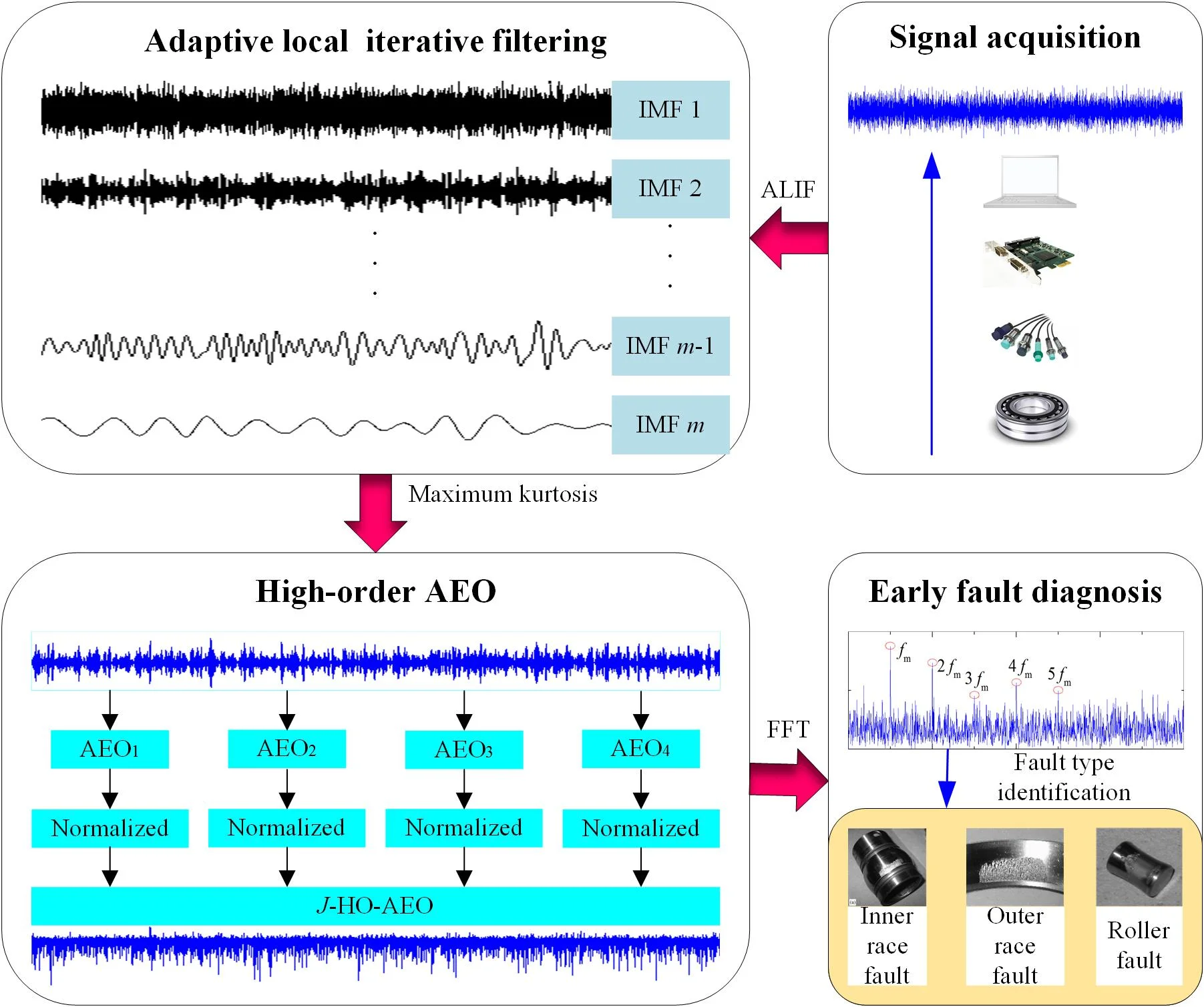
A framework based on ALIF and HO-AEO has been established for the early fault diagnosis of rolling bearings, and the steps are as follows:

(1) The faulty signals are collected and adaptive local iterative filtering is employed to decompose the faulty signals into a sum of IMFs.

(2) The optimal IMF is selected based on the maximum kurtosis with Eq. (22):

22

K u r t o s i s = \frac{N \sum_{i = 1}^{N} {(x_{i} - \bar{x})}^{4}}{{[\sum_{i = 1}^{N} {(x_{i} - \bar{x})}^{2}]}^{2}} .

Fig. 1Flowchart of bearing early fault diagnosis with HO-AEO improved by ALIF

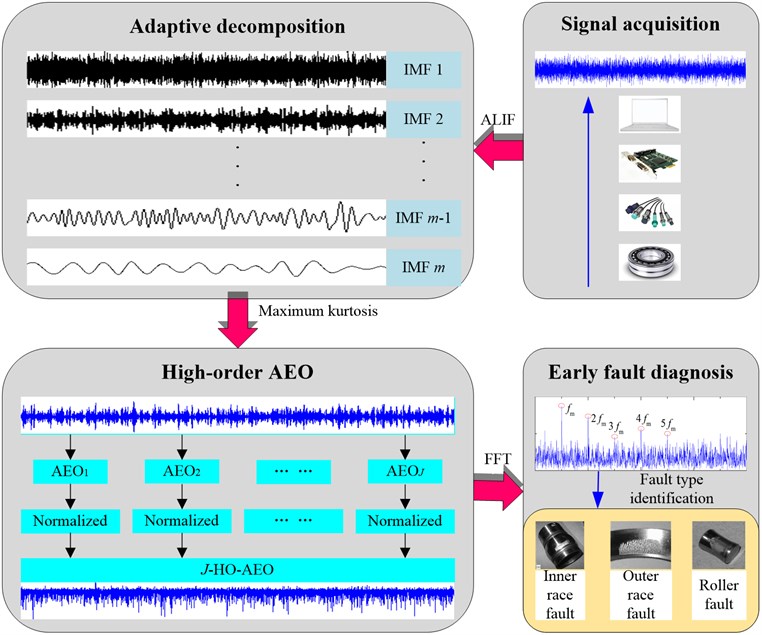
(3) Analytic energy operators from order 1 to $J$ are performed on the optimal IMF to enhance transient impulses, and in the following the multiple HO-AEO is computed with Eq. (19) and normalized with Eq. (21).

(4) Fast Fourier transform is utilized to the HO-AEO of the optimal IMF to obtain the higher-order analytical energy spectrum.

(5) The bearing fault is finally identified by the comparison between the prominent frequency in the higher-order analytical energy spectrum and the theoretic fault characteristic frequency of the faulty bearing.

The flowchart of the proposed approach is demonstrated in Fig. 1.

4.2. Simulation illustration

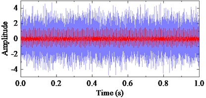
To verify the proposed approach in extracting the transient characteristics of the signal, a simulation test is performed. Because periodical impulses in the vibration signal of a defected bearing decay in the exponential type, the simulation signal with interference harmonics can be expressed by the following formula:

23

x (n) = A e^{- ξ ω_{r} (n - r f_{s} / f_{m}) / f_{s}} \sin [ω_{r} \frac{(n - r f_{s} / f_{m})}{f_{s}}] δ [\frac{(n - r f_{s} / f_{m})}{f_{s}}]

+ \sum_{k = 1}^{K} L_{k} \sin [ω_{k} \frac{(n - r f_{s} / f_{m})}{f_{s}}],

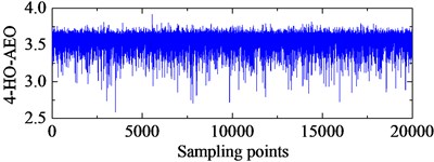
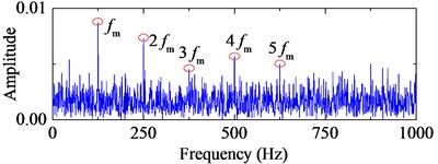
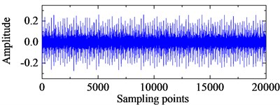
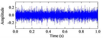
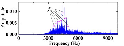
where $A$ is the amplitude of the impulse-induced vibration, $ξ$ is the damping characteristic factor, $ω_{r}$ is the excited resonance angular frequency, $f_{m}$ is the fault characteristic frequency, $f_{s}$ is the sampling frequency, and $δ (∙)$ is the Dirac function. In this simulation, parameters are set as: $A =$ 1.5, $ξ =$ 0.1, $f_{m} =$ 125 Hz, $f_{s} =$ 20000 Hz, $ω_{r} =$ 4000 $π$ rad/s. The interference harmonics are added with $L_{1} =$ 0.2, $ω_{1} =$ 426 $π$ rad/s and $L_{2} =$ 0.1, $ω_{2} =$ 1230 $π$ rad/s, respectively. The noise-contaminated signal is obtained by adding a Gaussian white noise with the SNR of –13 dB. A total of 20,000 samples are considered for the impulsive signal simulation as shown in Fig. 2 with the corresponding frequency spectrum by FFT.

Fig. 2The stimulated fault signals with periodic impulses and the corresponding frequency spectrum

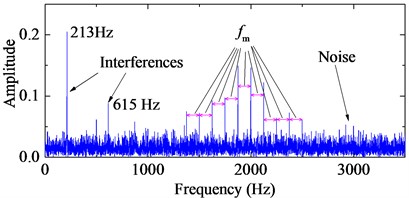
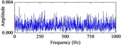
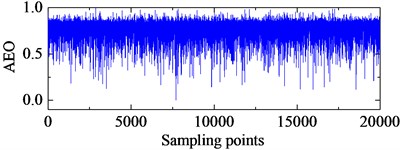
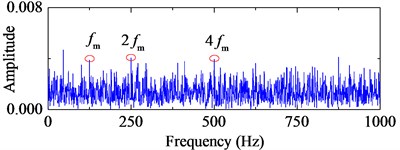
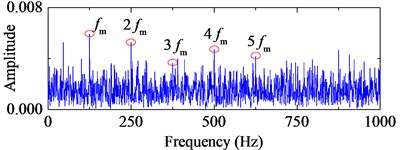
TEO, AEO and the corresponding 2-, 3-, 4-HO-AEO of the simulation signal are respectively shown in Fig. 3, as well as energy operator spectra of TEO, AEO and the 2-, 3-, 4-HO-AEO. From the comparison from Fig. 3(a) to Fig. 3(j), it can be seen that the operators are gradually away from the zero, namely, the negative limitation. In addition, fault characteristic frequency are submerged in the spectrum of the TEO in Fig. 3(b), hence it fails to diagnosis the fault. From the comparison of AEO and the corresponding 2-, 3-, 4-HO-AEO in Fig. 3(c) to Fig. 3(j), the fault characteristic frequency and its multiples are gradually distinct from AEO to the 4-HO-AEO. In addition, interference harmonics with 213 Hz and 615 Hz are removed. From the simulation analysis in [29], the fourth order AEO will be a better, hence the 4-HO-AEO is adopted in this paper for investigation of early bearing fault diagnosis. Nevertheless, the result of 4-HO-AEO is still not explicit due to the heavy noise. Hence, a pre-process with ALIF is introduced for low-pass filtering, and a comparison with EMD is performed. The convergence threshold $ε$ in ALIF is set as 0.001, and the convergence criterion of EMD is referred to [32].

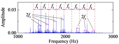
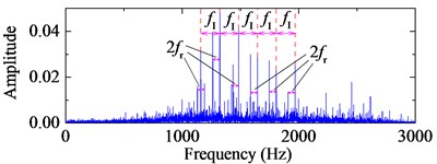
The first ten IMFs respectively with ALIF and EMD, with the corresponding frequency spectrum are shown in Fig. 4 and Fig. 5. Obviously, ALIF could get narrower frequency bands than EMD, which alleviate the mode mixing and will be more suitable for the 4-HO-AEO. The optimal IMF is obtained with the maximum kurtosis in Fig. 6. Based on the criteria, the fourth IMF in ALIF and the third IMF in EMD are selected. The optimal IMF by ALIF extracts more harmonic features in frequency domain than the one by EMD as shown in Fig. 7, meanwhile interference harmonics with 213 Hz and 615 Hz are efficiently separated by both ALIF and EMD, then type of the fault can be correctly identified.

Fig. 3Energy operators of the simulation signals and the corresponding frequency spectra

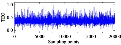
a) TEO of the simulation signal

b) Frequency spectrum of TEO

c) AEO of the simulation signal

d) Frequency spectrum of AEO

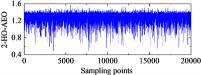
e) 2-HO-AEO of the simulation signal

f) Frequency spectrum of 2-HO-AEO

g) 3-HO-AEO of the simulation signal

h) Frequency spectrum of 3-HO-AEO

i) 4-HO-AEO of the simulation signal

j) Frequency spectrum of 4-HO-AEO

5. Experimental verification

To further investigate effectiveness and feasibility of the proposed approach for weak fault transient extraction, two experimental cases respectively with artificially seeded damage and run-to-failure are considered in this section.

Fig. 4IMFs by ALIF and the corresponding frequency spectra

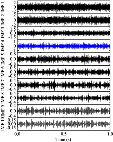
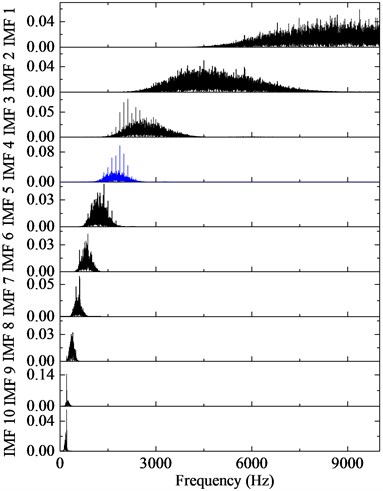
Fig. 5IMFs by EMD and the corresponding frequency spectra

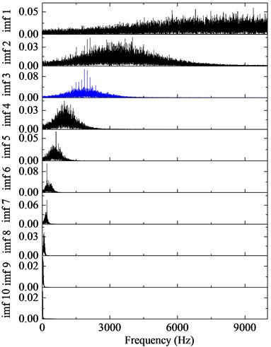
Fig. 6Kurtosis of IMFs with ALIF and EMD

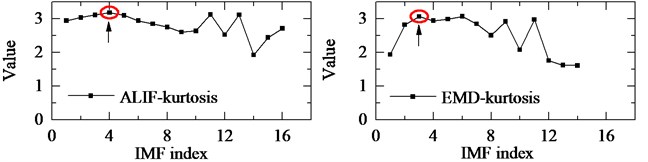
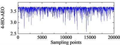
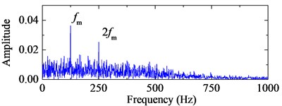
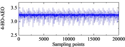
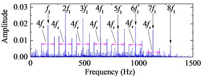
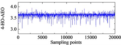
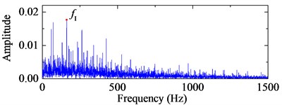
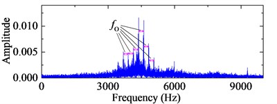
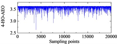
Fig. 74-HO-AEO with the optimal IMFs and the fault characteristic frequency spectra with ALIF and EMD

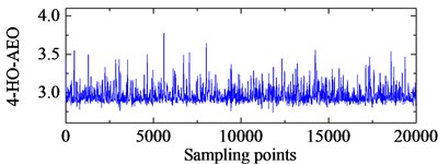
a) 4-HO-AEO of the fourth IMF in ALIF

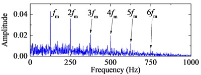
b) Frequency spectrum of the 4-HO-AEO with ALIF

c) 4-HO-AEO of the third IMF in EMD

d) Frequency spectrum of the 4-HO-AEO with EMD

5.1. Artificially seeded damage bearing with an inner race fault

The bearing data are downloaded from Bearing Data Centre of the Case Western Reserve University [33]. In this part, the drive end bearing with an inner race fault is investigated at speed of 1797 rpm. Since diameter of the fault in the inner race is 0.007 inch, this case can be treated as a slight fault. The fault characteristic frequency in theory can be calculated by Eq. (24) and Eq. (25).

Ball pass frequency on inner race (BPFI):

24

f_{I} = 0.5 z (1 + d \cos (\frac{α}{D})) f_{r} .

Ball pass frequency on outer race (BPFO):

25

f_{O} = 0.5 z (1 - d \cos (\frac{α}{D})) f_{r},

where $d$ is the diameter of the rolling element, $D$ is the pitch diameter, $α$ is the contact angle, $z$ is the number of rolling elements and $f_{r}$ the shaft speed.

Table 1Structural parameters of the drive end bearing and the characteristic frequency

$d$	$D$	$z$	$α$	$f_{r}$	$f_{I}$
7.94 mm	39.04 mm	9	0	29.95 Hz	162.19 Hz

The bearing type is 6205-2RS JEM SKF and its structural parameters with the corresponding characteristic frequency by Eq. (24) are listed in Table 1. The signal with 20000 points is shown in Fig. 8 with the sampling rate 12 kHz. Obviously, there is no fault characteristic frequency band in the spectrum. The third IMF in ALIF and the second one in EMD are respectively selected as the optimal IMFs according to the maximum kurtosis in Fig. 9. The selected IMF and the corresponding frequency spectra are shown in Fig. 10. Compared with the band in Fig. 10(d), a narrower frequency band with less noise interference is obtained in Fig. 10(b), and the interval frequency between two impulses are obvious. Hence the frequency band containing fault information can be extracted efficiently by ALIF compared with EMD. In the following, based on the 4-HO-AEO combined with the selected IMF by ALIF, the fault characteristic frequency with its multiples can be identified evidently in Fig. 11(b), but EMD in Fig. 11(d) fails to clearly show the fault characteristic frequencies due to the interference with heavy noise and harmonic waves.

Fig. 8The stimulated fault signals and the corresponding frequency spectrum

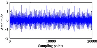
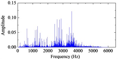
Fig. 9Kurtosis of IMFs with ALIF and EMD

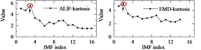
Fig. 10The optimal IMFs and the corresponding frequency spectra with ALIF and EMD

a) The third IMF in ALIF

b) Frequency spectrum of the third IMF in ALIF

c) The second IMF in EMD

d) Frequency spectrum of the second IMF in EMD

Fig. 114-HO-AEO of the optimal IMFs and the fault characteristic frequency spectra with ALIF and EMD

a) 4-HO-AEO of the third IMF in ALIF

b) Frequency spectrum of the 4-HO-AEO with ALIF

c) 4-HO-AEO of the second IMF in EMD

d) Frequency spectrum of the 4-HO-AEO with EMDs

5.2. Run-to-failure bearing with an outer race fault

The data are from Intelligent Maintenance System in University of Cincinnati. As shown in Fig. 12, bearing test rig comprises four bearings that are installed on one shaft. The rotation speed of shaft is controlled at 2000 rpm and a radial load of 6000 lb is placed on the shaft by a spring mechanism. The data length in the save file is 20,480 points with sampling rate 20 kHz. Rexnord ZA-115 double row bearings are used in the test with geometry parameters listed in Table 2. The fault characteristic frequency of the outer race is computed with Eq. (25). Details of the experiment could refer to [6].

Table 2Structural parameters of bearing Rexnord ZA-2115 and the characteristic frequency

$d$	$D$	$z$	$α$	$f_{r}$	$f_{O}$
8.4 mm	71.5 mm	16	15.17°	33.3 Hz	236.4 Hz

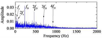
The bearing with outer race fault in the second group is selected for investigation. Kolmogorov-Smirnov (K-S) test statistic [34] is employed for monitoring the degradation path of the bearing in Fig. 13. Based on the degradation path, the faulty signal at an early time point 5400 min is selected for study. The original signal at 5400 min with its corresponding frequency spectrum are shown in Fig. 14. The first IMF in ALIF as well as in EMD is selected according to the maximum kurtosis in Fig. 15. Though the third IMF in the EMD kurtosis is larger than the first one, it fails to diagnosis the fault. The reason may be that it is a false IMF produced by EMD. The selected IMFs and the corresponding frequency spectra are shown in Fig. 16. The interference harmonic with frequency 985.2 Hz has been separated. Both fault characteristic frequency bands are obvious, but the noise in the low frequency domain of the band with ALIF is nearly removed compared with EMD, which means the influence of the noise will be slight for the fault characteristic frequency that are in the low frequency domain as well. The comparison between Fig. 17(b) and Fig. 17(d) shows the better capability of ALIF in enhancement of the fault characteristic frequency.

Fig. 12Illustration of bearing test rig with sensor placement

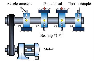
Fig. 13Bearing degradation path with K-S test statistic

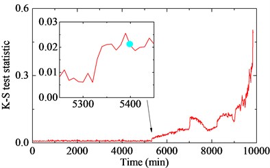
Fig. 14The stimulated fault signals and the corresponding frequency spectrum

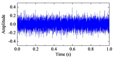
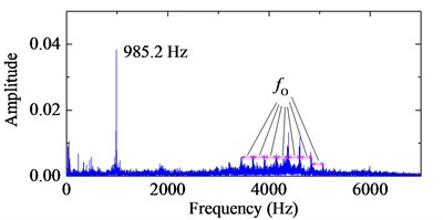
Fig. 15Kurtosis of IMFs with ALIF and EMD

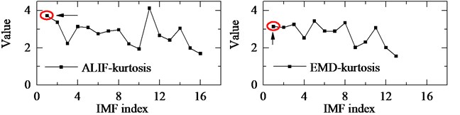
Fig. 16The optimal IMFs and the corresponding frequency spectra with ALIF and EMD

a) The first IMF in ALIF

b) Frequency spectrum of the first IMF in ALIF

c) The first IMF in EMD

d) Frequency spectrum of the first IMF in EMD

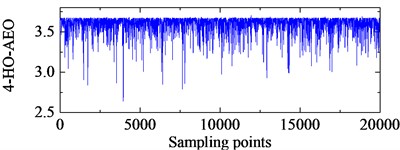
Fig. 174-HO-AEO of the optimal IMFs and the fault characteristic frequency spectra with ALIF and EMD

a) 4-HO-AEO of the first IMF in ALIF

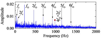
b) Frequency spectrum of the 4-HO-AEO with ALIF

c) 4-HO-AEO of the first IMF in EMD

d) Frequency spectrum of the 4-HO-AEO with EMD

6. Conclusions

In this paper, an improved HO-AEO based on ALIF is proposed for the early fault diagnosis in rolling element bearings. The approach could deal with non-stationary signals mixed with heavy noise in the operation of the fault bearing. The Teager energy operator could highlight the transient impulses in vibration signals of the faulty bearing. To more accurately extract the fault information, analytical energy operator with its high orders are developed. According to the comparison among TEO, AEO and 2-, 3- 4-HO-AEO in the simulation, the 4-HO-AEO is superior to the others in dealing with interferences and heavy noise.

To overcome the limitation of mono-component in energy operators and improve the diagnosis result, ALIF is utilized to decompose the nonlinear, non-stationary signals into multiple mono-components, and the resonance frequency band as the optimal IMF is selected with the maximum kurtosis. Then 4-HO-AEO is employed to enhance the transient impulses in the optimal IMF and the corresponding spectrum is obtained with FFT. The effectiveness of the proposed approach in the early fault diagnosis has been verified with the simulation study and two practical applications. Besides, ALIF outperforms EMD in terms of de-noising and elimination of mode mixing.

Since the proposed approach could perform well in experimental study considering heavy noise, then further studies could be extended to other mechanical parts like gears and practical applications. In addition, the band-filter is selected with the criteria of the maximum kurtosis, hence the other bands which contains fault information may be overlooked. Therefore, reconstruction of signals should be considered.

References

Randall R. B., Antoni J. Rolling element bearing diagnostics-a tutorial. Mechanical Systems and Signal Processing, Vol. 25, Issue 2, 2011, p. 485-520.

Publisher
Antoni J., Randall R. B. A stochastic model for simulation and diagnostics of rolling element bearings with localized faults. Journal of Vibration and Acoustics, Vol. 125, 2003, p. 282-289.

Publisher
Wei Y., Liu S. Numerical analysis of the dynamic behavior of a rotor-bearing-brush seal system with bristle interference. Journal of Mechanical Science and Technology, Vol. 33, Issue 8, 2019, p. 3895-3903.

Publisher
Feng Z., Liang M., Chu F. Recent advances in time-frequency analysis methods for machinery fault diagnosis: a review with application examples. Mechanical Systems and Signal Processing, Vol. 38, Issue 1, 2013, p. 165-205.

Publisher
Smith W. A., Randall R. B. Rolling element bearing diagnostics using the Case Western Reserve University data: a benchmark study. Mechanical Systems and Signal Processing, Vol. 64, Issue 65, 2015, p. 100-131.

Publisher
Qiu H., Lee J., Lin J., Yu G. Wavelet filter-based weak signature detection method and its application on roller bearing prognostics. Journal of Sound and Vibration, Vol. 289, Issues 4-5, 2006, p. 1066-1090.

Publisher
Wang Y., Xu G., Lin L., Jiang K. Detection of weak transient signals based on wavelet packet transform and manifold learning for rolling element bearing fault diagnosis. Mechanical Systems and Signal Processing, Vol. 54, Issue 55, 2015, p. 259-276.

Publisher
Lei Y., Lin J., He Z., Zi Y. Application of an improved kurtogram method for fault diagnosis of rolling element bearings. Mechanical Systems and Signal Processing, Vol. 25, Issue 5, 2011, p. 1738-1749.

Publisher
Feng Z., Zhang D., Zuo M. J. Adaptive mode decomposition methods and their applications in signal analysis for machinery fault diagnosis: a review with examples. IEEE Access, Vol. 5, 2017, p. 24301-24331.

Publisher
Huang N. E., Shen Z., Long S. R., Wu M. C., Shih H. H., Zheng Q., Yen N. C., Tung C. C., Liu H. H. The empirical mode decomposition and the Hilbert spectrum for nonlinear and non-stationary time series analysis. Proceedings of the Royal Society A: Mathematical, Physical and Engineering Sciences, Vol. 454, Issue 1971, 1998, p. 903-995.

Publisher
Cheng J., Yu D., Yu Y. The application of energy operator demodulation approach based on EMD in machinery fault diagnosis. Mechanical Systems and Signal Processing, Vol. 21, Issue 2, 2007, p. 668-677.

Publisher
Lei Y., Lin J., He Z., Zuo M. A review on empirical mode decomposition in fault diagnosis of rotating machinery. Mechanical Systems and Signal Processing, Vol. 35, Issues 1-2, 2013, p. 108-126.

Publisher
Feng Z., Zuo M. J., Hao R., Chu F., Lee J. Ensemble empirical mode decomposition-based Teager energy spectrum for bearing fault diagnosis. Journal of Vibration and Acoustics, Vol. 135, Issue 3, 2013, p. 031013.

Publisher
Kedadouche M., Thomas M., Tahan A. A comparative study between empirical wavelet transforms and empirical mode decomposition methods: application to bearing defect diagnosis. Mechanical Systems and Signal Processing, Vol. 81, 2016, p. 88-107.

Publisher
Zhu J., Wang C., Hu Z., Kong F., Liu X. Adaptive variational mode decomposition based on artificial fish swarm algorithm for fault diagnosis of rolling bearings. Proceedings of the Institute of Mechanical Engineering, Part C: Journal of Mechanical Engineering Sciences, Vol. 231, Issue 4, 2017, p. 635-654.

Publisher
Cicone A., Liu J., Zhou H. Adaptive local iterative filtering for signal decomposition and instantaneous frequency analysis. Applied Computational Harmonic Analysis, Vol. 41, Issue 2, 2016, p. 384-411.

Publisher
Feng Z., Chu F., Zuo M. J. Time-frequency analysis of time-varying modulated signals based on improved energy separation by iterative generalized demodulation. Journal of Sound and Vibration, Vol. 330, Issue 6, 2011, p. 1225-1243.

Publisher
Wei D., Jiang H., Shao H., Li X., Lin Y. An optimal variational mode decomposition for rolling bearing fault feature extraction. Measurement Science and Technology, Vol. 30, Issue 5, 2019, p. 055004.

Publisher
Piersanti M., Materassi M., Cicone A., Spogli L., Zhou H., Ezquer R. G. Adaptive local iterative filtering: a promising technique for the analysis of non-stationary signals. Journal of Geophysical Research: Space Physical, Vol. 123, Issue 1, 2018, p. 1031-1046.

Search CrossRef
Yang D., Wang B., Cai G., Wen J. Oscillation mode analysis for power grids using adaptive local iterative filter decomposition. International Journal of Electrical Power and Energy System, Vol. 92, 2017, p. 25-33.

Publisher
An X., Zeng H., Li C. Demodulation analysis based on adaptive local iterative filtering for bearing fault diagnosis. Measurement, Vol. 94, 2016, p. 554-560.

Publisher
Boudraa A. O., Salzenstein F. Teager-Kaiser energy methods for signal and image analysis: a review. Digital Signal Processing, Vol. 78, 2018, p. 338-375.

Publisher
Potamianos A., Maragos P. A comparison of the energy operator and the Hilbert transform approach to signal and speech demodulation. Signal Processing, Vol. 37, Issue 1, 1994, p. 95-120.

Publisher
Maragos P., Kaiser J. F., Quatieri T. F. Energy separation in signal modulations with application to speech analysis. IEEE Transactions on Signal Processing, Vol. 41, Issue 10, 1993, p. 3024-3051.

Publisher
Maragos P., Kaiser J. F., Quatieri T. F. On amplitude and frequency demodulation using energy operators. IEEE Transactions on Signal Processing, Vol. 41, Issue 4, 1993, p. 1532-1550.

Publisher
Liang M., Faghidi H. Intelligent bearing fault detection by enhanced energy operator. Expert System with Applications, Vol. 41, Issue 16, 2014, p. 7223-7234.

Publisher
Zeng M., Yang Y., Zheng J., Cheng J. Normalized complex Teager energy operator demodulation method and its application to fault diagnosis in a rubbing rotor system. Mechanical Systems and Signal Processing, Vol. 50, Issue 51, 2015, p. 380-399.

Publisher
Imaouchen Y., Kedadouche M., Alkama R., Thomas M. A frequency-weighted energy operator and complementary ensemble empirical mode decomposition for bearing fault detection. Mechanical Systems and Signal Processing, Vol. 82, 2017, p. 103-116.

Publisher
Faghidi H., Liang M. Detection of bearing fault detection from heavily contaminated signals: a higher-order analytic energy operator method. Journal of Vibration and Acoustics, Vol. 137, Issue 4, 2015, p. 041012.

Publisher
Maragos P., Potamianos A. Higher order differential energy operators. IEEE Signal Process Letters, Vol. 2, Issue 8, 1995, p. 152-154.

Publisher
Salzenstein F., Boudraa A. O., Cexus J. C. Generalized higher-order nonlinear energy operators. Journal of the Optical Society of America, Vol. 24, Issue 12, 2007, p. 3717-3727.

Publisher
Rilling G., Flandrin P., Gonçalves P. On empirical mode decomposition and its algorithms. IEEE-EURASIP Workshop Nonlinear Signal Image Processing, 2003, p. 8-11.

Publisher
Case Western Reserve University, Bearing Data Center. Available online: http://csegroups.case.edu /bearingdatacenter/pages/apparatus-procedures.

Search CrossRef
Cong F., Chen J., Pan Y. Kolmogorov-Smirnov test for rolling bearing performance degradation assessment and prognosis. Journal of Vibration and Control, Vol. 17, Issue 9, 2010, p. 1337-1347.

Publisher

Cited by

An integrated monitoring scheme for wind turbine main bearing using acoustic emission

Zhipeng Ma | Ming Zhao | Mourui Luo | Chao Gou | Guanji Xu

(2023)

Fault feature extraction of rolling element bearings based on short-time processing

Fan Chen

(2022)

Integrated early fault diagnosis method based on direct fast iterative filtering decomposition and effective weighted sparseness kurtosis to rolling bearings

(2022)

Compound Fault Diagnosis of Rolling Bearing Based on ALIF-KELM

Jie Ma | Shitong Liang | Zhengyu Du | Ming Chen | Yong Chen

(2021)

Early fault diagnosis of rolling bearings based on signal reconstruction through SDD-SVD and FWEO

Tiangang Zou | Jinbao Zhang | Yadong Sun | Zhenqiong Zheng | Yutong Guo

(2021)

About this article

Received

12 May 2019

Accepted

16 September 2019

Published

15 February 2020

SUBJECTS

Fault diagnosis based on vibration signal analysis

DOI

https://doi.org/10.21595/jve.2019.20794

Keywords

early fault diagnosis

rolling bearing

higher-order analytic energy operator

adaptive local iterative filtering

Acknowledgements

This work was supported by the National Natural Science Foundation of China (Grant No. 51505100). The authors would like to thank the editors and the anonymous reviewers for their valuable suggestions which have greatly improved the paper.

This is an open access article distributed under the Creative Commons Attribution License, which permits unrestricted use, distribution, and reproduction in any medium, provided the original work is properly cited.

Previous article in issue Previous Next article in issue Next

Research article

2023 10 09

Extraction and diagnosis of rolling bearing fault signals based on improved wavelet transform

Zhiqing Cheng

Research article

2023 08 01

Motor rolling bearing fault diagnosis based on MVMD energy entropy and GWO-SVM

Jian Tang, Qiaoni Zhao

Research article

2021 02 04

Research on fault diagnosis of rolling bearings based on conditional variance statistic and cross-correlation spectrum

Baoyu Huang, Yongxiang Zhang, Danchen Zhu

Research article

2019 11 15

Novel complete ensemble EMD with adaptive noise-based hybrid filtering for rolling bearing fault diagnosis

Xiaojun Song, Hongwei Sun, Liwei Zhan

J. Zhang, Y. Zhao, M. Liu, and L. Kong, “An improved higher-order analytical energy operator with adaptive local iterative filtering for early fault diagnosis of bearings,” Journal of Vibroengineering, Vol. 22, No. 1, pp. 67–82, Feb. 2020, https://doi.org/10.21595/jve.2019.20794

Copy Extrica

Copied to clipboard!

TY  - JOUR
DO  - 10.21595/jve.2019.20794
UR  - https://doi.org/10.21595/jve.2019.20794
TI  - An improved higher-order analytical energy operator with adaptive local iterative filtering for early fault diagnosis of bearings
T2  - Journal of Vibroengineering
AU  - Zhao, Yongqiang
AU  - Zhang, Jinbao
AU  - Liu, Ming
AU  - Kong, Lingxian
PY  - 2020
DA  - 2020/02/15
PB  - JVE International Ltd.
SP  - 67-82
IS  - 1
VL  - 22
SN  - 1392-8716
SN  - 2538-8460
ER  - 

Copy Ris

Copied to clipboard!

@article{Zhao_2020,
	doi = {10.21595/jve.2019.20794},
	url = {https://doi.org/10.21595/jve.2019.20794},
	year = 2020,
	month = {feb},
	publisher = {{JVE} International Ltd.},
	volume = {22},
	number = {1},
	pages = {67--82},
	author = {Yongqiang Zhao and Jinbao Zhang and Ming Liu and Lingxian Kong},
	title = {An improved higher-order analytical energy operator with adaptive local iterative filtering for early fault diagnosis of bearings},
	journal = {Journal of Vibroengineering}
}

Copy Bibtex

Copied to clipboard!

[1]Y. Zhao, J. Zhang, M. Liu, and L. Kong, “An improved higher-order analytical energy operator with adaptive local iterative filtering for early fault diagnosis of bearings,” Journal of Vibroengineering, vol. 22, no. 1, pp. 67–82, Feb. 2020, doi: 10.21595/jve.2019.20794.

Copy IEEE

Copied to clipboard!

Zhao, Yongqiang, Jinbao Zhang, Ming Liu, and Lingxian Kong. “An Improved Higher-Order Analytical Energy Operator with Adaptive Local Iterative Filtering for Early Fault Diagnosis of Bearings.” Journal of Vibroengineering 22, no. 1 (February 15, 2020): 67–82. https://doi.org/10.21595/jve.2019.20794.

Copy Chicago

Copied to clipboard!

An improved higher-order analytical energy operator with adaptive local iterative filtering for early fault diagnosis of bearings

Abstract

Highlights

1. Introduction

2. Adaptive local iterative filtering

3. High-order analytical energy operator

3.1. Teager energy operator

3.2. Analytic energy operator

3.3. Higher-order analytic energy operator

4. The proposed method with a simulation illustration

4.1. The proposed method

4.2. Simulation illustration

5. Experimental verification

5.1. Artificially seeded damage bearing with an inner race fault

5.2. Run-to-failure bearing with an outer race fault

6. Conclusions

References

Cited by

About this article

Related Articles