Chaotic time series prediction using wavelet transform and multi-model hybrid method

Feng, Tian; Yang, Shuying; Han, Feng

doi:10.21595/jve.2019.20579

Journal of Vibroengineering

Browse Journal

Submit article

Published: 15 November 2019

Check for updates

Chaotic time series prediction using wavelet transform and multi-model hybrid method

Tian Feng¹

Shuying Yang²

Feng Han³

¹School of Computer Science and Engineering, Tianjin University of Technology, Tianjin, 300384, China

^{2, 3, 1}Key Laboratory of Computer Vision and System, Ministry of Education, Tianjin, 300384, China

Corresponding Author:

Tian Feng

Cite the article Download PDF

Downloads 1702

WoS Core Citations 6

CrossRef Citations 9

Abstract

In order to further improve the prediction accuracy of the chaotic time series and overcome the defects of the single model, a multi-model hybrid model of chaotic time series is proposed. First, the Discrete Wavelet Transform (DWT) is used to decompose the data and obtain the approximate coefficients (low-frequency sequence) and detailed coefficients (high-frequency sequence) of the sequence. Secondly, phase space reconstruction is performed on the decomposed data. Thirdly, the chaotic characteristics of each sequence are judged by correlation integral and Kolmogorov entropy. Fourthly, in order to explore the deeper features of the time series and improve the prediction accuracy, a sequence of Volterra adaptive prediction models is established for the components with chaotic characteristics according to the different characteristics of each component. For the components without chaotic characteristics, a JGPC prediction model without chaotic feature sequences is established. Finally, the multi-model fusion prediction of the above multiple sequences is carried out by the LSTM algorithm, and the final prediction result is obtained through calculation, which further improves the prediction accuracy. Experiments show that the multi-model hybrid method of Volterra-JGPC-LSTM is more accurate than other comparable models in predicting chaotic time series.

1. Introduction

Chaotic time series are highly non-linear, uncertain and random, etc., and it is difficult to master the change rules and characteristics of conventional analysis and prediction methods, making it a difficult problem to make an accurate prediction of time series [1]. Over the years, many researchers have studied and developed various prediction models, among which GPC, Volterra model and ANN have been widely used [2, 3]. Generalized predictive control (GPC) algorithm in predictive control can effectively solve multi-step prediction, and combines with identification and self-tuning mechanism, and combines the identification and self-correction mechanism to predict chaotic time series. It has strong robustness and can effectively overcome system lag [4]. In recent years, with the progress and development of functional theory, the Volterra filter has received extensive attention due to its advantages of fast training speed, strong nonlinear approximation ability and high prediction accuracy [5, 6]. Although ANN has strong nonlinear approximation ability and self-learning ability, it has been widely used in the field of financial time series prediction [7]. However, some studies have shown that ANN has some limitations, such as that it is easy for ANN to fall into a local minimum during training, and it is easy to produce overfitting phenomenon and slow convergence speed [8]. The prediction accuracy of a single model for chaotic time series cannot meet the actual requirements, and the mixed prediction model shows greater advantages compared with the single prediction model. The CAO method [9] proposed by Liangyue Cao can not only calculate the embedding dimension of time series but also can be used for time series chaotic characteristics analysis [10], which is very helpful for our proposed hybrid prediction model. Literature [11] proposed a genetic algorithm for wind power prediction-Volterra neural network (GA-VNN) model, which combines the structural features of the Volterra functional model and BP neural network model, and uses genetic algorithm to improve the combined model. The global optimization ability, in the wind power ultra-short-term multi-step prediction, its prediction performance is significantly higher than the Volterra model and the BP neural network model, but the combined model has a shorter prediction step size, greater application limitations, complex structure, and computational complexity. In order to obtain more detailed information on the time series, it is necessary to construct different prediction models for sequences with different characteristics. Establishing appropriate prediction models for the decomposed sequences can improve the prediction accuracy. Wavelet analysis is a time-frequency analysis method developed in recent years. It has good localization properties for signals and can extract any details of signals, which provides a new method for preprocessing of non-stationary time series data. In the literature [12], the wavelet transform is used in chaotic time series. Literature [13, 14] proposes a method of wavelet transform and multi-model fusion to predict time series. In the literature [15], the wavelet transform and the cyclic neural network model are used to decompose the watermark time series, and then the decomposed data are separately modeled and predicted. Literature [16] proposes a hybrid model combining the ARIMA model with an artificial neural network (ANN) and fuzzy logic for stock forecasting. Literature [17] proposed a wavelet and autoregressive moving average (ARMA) model for predicting the monthly discharge time series. The main advantage of wavelet analysis over traditional methods is the ability to convert raw complex series to different frequencies and times [18]. Each component can be studied with a resolution that matches its scale, which is especially useful for complex time-series predictions. All of the above methods simply use the wavelet transform to decompose the time series. Instead of performing the time series analysis and judgment on the decomposed prediction, the same side model is directly established, and the predicted results are directly accumulated as the final predicted value. However, the method is that the results of each model prediction are directly superimposed so that the prediction error of each prediction model can be accumulated to the final prediction value, and the prediction accuracy cannot be further improved. Therefore, in order to solve the problem of error accumulation, the wavelet decomposition sequence should judge the chaotic characteristics and stationarity of the wavelet decomposition sequence, and then model the prediction. The final model fusion prediction for each model prediction value is very necessary.

Since the JGPC model only has high prediction accuracy for non-chaotic time series, the Volterra model only has high prediction accuracy for the chaotic time series. Therefore, in order to further improve the prediction accuracy of the chaotic time series, a hybrid Volterra-JGPC-LSTM model is proposed to predict the chaotic time series. Firstly, the data is decomposed by a discrete wavelet transform (DWT) to obtain the approximate coefficients (low-frequency sequence) and detail coefficients (high-frequency sequence) of the sequence, and then the coefficients are reconstructed separately. Secondly, phase space reconstruction is performed on the low-frequency sequence and each high-frequency sequence respectively. Thirdly, the chaotic characteristics of each sequence are determined by correlation integral and Kolmogorov entropy. Fourthly, the Volterra adaptive prediction model is established for the sequences with chaotic characteristics, and the JGPC prediction model is established for the sequences without chaotic characteristics. Finally, when calculating the final predicted value, this paper does not directly accumulate the prediction of each part but uses the LSTM algorithm to perform multi-model fusion prediction on the above sequence. The combined prediction error is smaller than the single model prediction error, which further improves the prediction accuracy.

2. Chaotic time series decomposition based on Mallat discrete wavelet transform

As a non-stationary signal processing method based on time and scale, the wavelet transform has good localization characteristics in both time domain and frequency domain. Multi-scale detailed analysis of the signal by functions such as stretching and translation can effectively eliminate noise in financial time series and fully retain the characteristics of the original signal [19]. For Discrete financial time series data, scaling factor a and moving factor b need to be discretized respectively to obtain Discrete Wavelet Transform (DWT).

If $a = {a_{0}}^{j}$ , $b = k {a_{0}}^{j} b_{0}$ , $k, j \in Z$ , then the discrete wavelet function is:

1

ψ_{j, k} (t) = {a_{0}}^{- \frac{j}{2}} ψ ({a_{0}}^{- j} t - k b_{0}) .

Then the corresponding discrete wavelet transform is:

2

W T_{f} (a, b) = \int_{- \infty}^{+ \infty} x (t) {\bar{ψ}}_{j . k} (t) d t .

In Eqs. (1) and (2), wavelet analysis can obtain the low-frequency or high-frequency information of the financial time series data signal by increasing or decreasing the scaling factor a, so as to analyze the contour of the sequence signal or the details of the information. Mallat algorithm is a fast wavelet transform algorithm for layer by layer decomposition and reconstruction based on multi-resolution analysis, which greatly reduces the matrix operation time and complexity in signal decomposition [20]. Therefore, the fast discrete wavelet transforms the Mallat algorithm is adopted in this paper to decompose and reconstruct the financial time series, reduce the impact of short-term noise interference on the structure of the neural network, and improve the predictive ability of the model. The wavelet decomposition and reconstruction of discrete financial time series signal $y$ can be realized in the form of subband filtering [21]. The formula of signal decomposition is as follows:

3

\begin{array}{l} c_{j + 1} (t) = \sum_{n \in z} c_{j} (n) F_{0} (n - 2 t), \\ d_{j + 1} (t) = \sum_{n \in z} c_{j} (n) F_{1} (n - 2 t) . \end{array}

The formula for signal reconstruction is:

4

c_{j} (t) = \sum_{n \in t} c_{j + 1} (n) F (t - 2 n) + d_{j + 1} (m) F_{1} (t - 2 n) .

The low-frequency part of the financial time series obtained by discrete wavelet transform reflects the overall trend of the series while the high-frequency part reflects the short-term random disturbance of the series. Daubechies wavelet has good characteristics for non-stationary time series. In order to ensure real-time and prediction accuracy, the 5-layer db6 wavelet is adopted in this paper for decomposition and reconstruction. In order to achieve the purpose of noise removal, the single-branch reconstruction of Mallat wavelet is carried out according to the low-frequency coefficients of layer 6 and the high-frequency coefficients of layer 1 to 5. Different high-frequency and low-frequency sequences can be obtained, and the preprocessed data is reconstructed in phase space as the training data of the subsequent model.

3. Judgment of chaotic characteristics

3.1. Phase space reconstruction

The analysis and prediction of chaotic time series are carried out in phase space. Phase space reconstruction is the premise and basis for studying and analyzing chaotic dynamic systems. Therefore, phase space reconstruction of financial time series is the first step to analyze chaotic characteristics [22], which can construct a one-dimensional time series from the high-dimensional phase space structure of the original system. In the high-dimensional phase space, many important characteristics such as the attractor of the chaotic dynamic system are preserved, which fully shows one Multiple layer of unknown information contained in a dimensional sequence. According to the embedding theorem of Takens, for any time series, as long as the appropriate embedding dimension m and the correlation dimension d of the dynamical system, i.e. $m \geq 2 d + 1$ are selected, the multi-dimensional spatial attractor trajectory of the sequence can be restored, and the phase space dimension of the studied time series is expanded. The reconstructed phase space will have the same geometric properties as the prime mover system and be equivalent to the prime mover system in the topological sense [23]. For a given univariate time series $x (i)$ , $i = 1,2, \dots, N$ , $N$ is the total length of the sequence. Then the reconstructed phase space is:

5

[\begin{matrix} x (1) & x (2) & \dots & x (M) \\ x (1 + τ) & x (2 + τ) & \dots & x (M + τ) \\ ⋮ & ⋮ & ⋮ & ⋮ \\ x [1 + (m - 1) τ] & x [2 + (m - 1) τ] & \dots & x [M + (m - 1) τ] \end{matrix}],

where $m$ is the embedded dimension and $τ$ is the delay time. The phase points in the phase space are expressed as: $X_{i} = [x (i), x (i + τ), \dots, x (i + (m - 1) τ)],$ where $i = 1,2, \dots, M,$ $M = N - (m - 1) τ$ . The key to phase space reconstruction is to choose the appropriate delay time $τ$ and embedding dimension $m$ . The two methods for calculating the delay time are the autocorrelation method, the complex correlation method, and the mutual information method. The method of calculating the embedding dimension m has the correlation dimension. Law, false neighbors and the CAO method. In this paper, the mutual information method is used to find the delay time $τ$ , and the CAO method is used to find the embedding dimension [9]. The mutual information method overcomes the shortcomings of the autocorrelation method and can be extended to the high-dimensional nonlinear problem. It is an effective method for calculating the delay time in phase space reconstruction. The CAO method overcomes the problem of judging the true neighbor and the false neighbor in the pseudo nearest neighbor method. The disadvantage of choosing a threshold.

3.2. Judging the chaotic characteristics of Kolmogorov entropy

$K$ entropy is a kind of commonly used soil, which is evolved based on thermodynamic soil and information soil, and reflects the motion property and state of the dynamic system. It is used to represent the degree of chaos in the movement of the system. It represents the degree of loss of system information and is commonly used to measure the degree of chaos or disorder in the operation of the system [24]. The $K_{2}$ entropy proposed by Grassberger and Procaccia has the following relationship with the correlation integral $C_{m}^{2} (ε)$ :

6

K_{2} = \frac{1}{τ} l o g_{2} \frac{C_{m}^{2} (ε)}{C_{m + 1}^{2} (ε)} .

When $m$ reaches a certain value, $K_{2}$ tends to be more stable, and the relatively stable $K_{2}$ can be used as an estimate of $K$ . According to the above discussion, under the condition that the embedding dimension increases continuously at the same interval, an equal slope linear regression is made on the point in the dual-logarithmic coordinate $l n C_{m}^{2} (ε) ~ l n ε$ in the scale-free interval, and the stability estimation of correlation and $K$ can be obtained simultaneously [25]. Kolmogorov entropy $K$ plays an important role in the measurement of chaos. It can be used to judge the nature of system motion. For regular motion, $K =$ 0. In a stochastic system, $K$ goes to $\infty$ . If the system presents deterministic chaos, $K$ is a constant greater than zero. The higher the K entropy is, the higher the loss rate of information is, the more chaotic the system is, or the more complex the system is.

4. Multi-model fusion method based on Volterra-JGPC-LSTM

4.1. An improved generalized predictive control model (JGPC)

Generalized predictive control (JGPC) algorithm is a predictive control method developed on the basis of adaptive control research. In the JGPC algorithm, the controlled autoregressive integral moving average model (CARIMA) in the minimum variance control is used to describe the random disturbance object. Generalized predictive control (JGPC) uses the following discrete difference equations with stochastic step disturbance to describe the mathematical model of the controlled plant:

7

A (z^{- 1}) y (k) = B (z^{- 1}) u (k - 1) + C (z^{- 1}) \frac{ξ (k)}{Δ} .

The above formula is equivalent to:

8

Δ y (k) = [A (z^{- 1}) - 1] [- Δ y (k)] + B (z^{- 1}) Δ u (k - 1) + C (z^{- 1}) ξ (k) = φ^{T} (k) θ + ξ (k) .

In the formula:

φ^{T} (k) = [- Δ y (k - 1), - Δ y (k - 2), \dots, - Δ y (k - n_{a}), Δ u (k - 1), Δ u (k - 2), \dots,

Δ u (k - n_{b} - 1), ξ (k - 1), ξ (k - 2), \dots, ξ (k - n_{c})],

\hat{θ} = [{\hat{a}}_{1}, {\hat{a}}_{2}, \dots, {\hat{a}}_{n_{a}}, {\hat{b}}_{0}, {\hat{b}}_{1}, \dots, {\hat{b}}_{n_{b}}, {\hat{c}}_{1}, {\hat{c}}_{2}, \dots, {\hat{c}}_{n_{c}}]^{T},

Δ y (k) = y (k) - y (k - 1), Δ = 1 - z^{- 1} .

Then the recursive least squares formula is:

9

\begin{array}{l} \hat{θ} (k) = \hat{θ} (k - 1) + K (k) [Δ y (k) - φ^{T} (k) \hat{θ} (k - 1)], \\ K (k) = \frac{P (k - 1) φ (k)}{λ + φ^{T} (k) P (k - 1) φ (k)}, \\ P (k) = \frac{1}{λ} [I - K (k) φ^{T} (k)] P (k - 1) . \end{array}

Recursive by Eq. (13), the system’s minimum variance output prediction model at the future time is:

10

\hat{Y} = G Δ U + Y_{m} .

In the formula:

11

\{\begin{array}{l} \hat{Y} = [\hat{y} (k + d| k), \hat{y} (k + d + 1| k), \dots, \hat{y} (k + N| k)]^{T}, \\ Y_{m} = [y_{m} (k + d), y_{m} (k + d + 1), \dots ， y_{m} (k + N)]^{T}, \\ Δ U = [Δ u (k), Δ u (k + 1), \dots, Δ u (k + N - d)]^{T}, \\ G = {[\begin{matrix} g_{1,0} & 0 & \dots & 0 \\ g_{2,0} & g_{1,0} & \dots & 0 \\ ⋮ & ⋮ & g_{1,0} & ⋮ \\ g_{N - d + 1,0} & g_{N - d, 0} & \dots & g_{1,0} \end{matrix}]}_{(N - d + 1) \times (N - d + 1)}, \end{array}

where $N$ is the predicted length.

The $G$ matrix element in Eq. (11) can be calculated by the following formula:

12

\begin{array}{l} g_{j, 0} = b_{1, j - 1} - \sum_{i = 1}^{j_{1}} a_{1, i} g_{j - i, 0}, \\ j = 2,3, \dots N - d + 1, j_{1} = m i n \{j - 1, n_{a}\} . \end{array}

$y_{m} (k + j)$ can be determined by past control inputs and outputs, which can be derived from:

13

y_{m} (k + j) = - \sum_{i = 1}^{n_{a}} a_{1, i} y_{m} (k + j - i) + \sum_{j = 0}^{n_{b}} b_{1, j} u (k + j - d - i | k)

+ \sum_{i = 0}^{n_{c}} c_{1, i} ω (k + j - i | k), j = 1,2, \dots, N .

In addition, let the reference trajectory by:

14

\{\begin{array}{l} y_{r} (k + d - 1) = y_{m} (k + d - 1), \\ y_{r} (k + d + i) = α y_{r} (k + d + i - 1) + (1 - α) ω (k + d), \\ Y_{r} = [y_{r} (k + d), y_{r} (k + d + 1), \dots, y_{r} (k + N)] . \end{array}

In the formula, $ω (k + d)$ is the expected output at time $k$ , $α$ is the output softening coefficient, and $Y_{r}$ is the reference trajectory vector.

The task of generalized predictive control is to make the output $Y$ of the controlled object as close as possible to $Y_{r}$ . Therefore, the performance indicator function is defined as follows:

15

J = E {(Y - Y_{r})^{T} (Y - Y_{r}) + Δ U^{T} Γ Δ U\} .

In the formula, $Γ$ is usually a unit array, obtain the corresponding JGPC control law as:

16

Δ U = {(G^{T} G + Γ)}^{- 1} G^{T} (Y_{r} - Y_{m}) .

For the multi-step prediction of high-dimensional chaotic systems, a large number of practices show that JGPC has high prediction accuracy and prediction efficiency, so it can be used to construct a multi-step prediction model of chaotic time series.

4.2. Volterra chaotic time series adaptive prediction model

Volterra functional series can usually describe the nonlinear behavior of response and memory functions, and it can approximate the arbitrary continuous function with arbitrary precision. For the nonlinear systems, the Volterra-based adaptive prediction filter method can feedback iterative adjustment on the parameters of the filter, so as to realize the optimal filter [26].

Nonlinear dynamic system input is expressed as $X (t) = [x (t), x (t - 1), \dots, x (t - N + 1)]$ , the output is indicated as $Y (n) = x (n + 1)$ . Nonlinear dynamical system of Volterra expansions is represented as follows:

17

x (t + 1) = F (X (t)) = h_{0} + \sum_{m = 0}^{+ \infty} h_{1} (m) x (t - m)

+ \sum_{m_{1} = 0}^{+ \infty} \sum_{m_{2} = 0}^{+ \infty} h_{2} (m_{1}, m_{2}) x (t - m_{1}) x (t - m_{2}) + \dots

+ \sum_{m_{1} = 0}^{+ \infty} \sum_{m_{2} = 0}^{+ \infty} \dots \sum_{m p = 0}^{+ \infty} h_{p} (m_{1}, m_{2}, \dots, m_{p}) x (t - m_{1}) x (t - m_{2}) \dots x (t - m_{p}) + \dots,

where $h_{1}$ , $h_{2}$ ,..., $h_{n}$ is the kernel function in the Volterra series, it is an implicit function of the system, and reflects the macroscopic of the speech signal, $p$ is the filter length. According to the characteristics of voice time series, to reduce the amount of computation, the second-order Volterra adaptive prediction model usually is selected to truncated forms of expression as follows:

18

\hat{x} (t + 1) = h_{0} + \sum_{i_{1} = 0}^{N - 1} h_{1} (i_{1}) x (t - i_{1} τ) + \sum_{i_{1}, i_{2} = 0}^{N - 1} h_{2} (i_{1}, i_{2}) x (t - i_{1} τ) x (t - i_{2} τ) .

Through the Volterra series expansion of the chaotic time series, the case is $m$ -item second-order Volterra filter cut-off ( $m$ is the minimum embedding dimension for chaotic time series). Through the state extension, the total number of the system is $M = 1 + m + m (m - 1) / 2$ , the filter coefficient vector and the input vector are respectively as follows:

19

\begin{matrix} H (t) = [h_{0}, h (0), h (1), \dots, h (m - 1), h_{2} (0,0), {h_{2} (0,1), \dots, h_{2} (t - m + 1)]}^{T}, \end{matrix}

20

\begin{matrix} U (n) = [1, x (n), x (n - 1), \dots, x (n - m + 1), x^{2} (n), {x (n) x (n - 1), \dots, x^{2} (n - m + 1)]}^{T} . \end{matrix}

Since the Volterra adaptive filter coefficients can be directly determined by linear adaptive FIR filter algorithm, the Eq. (18) can be expressed as:

21

\hat{x} (t + 1) = H^{T} (t) U (t) .

The Volterra adaptive process can adapt to the input and noise unknown or time-varying system characteristics. The principle of adaptive filtering is to iteratively feedback the filter parameters at the current moment by the error of the filter parameters obtained at the previous time, so as to achieve the most parameters. Excellent, and then achieve optimal filtering. The advantage of the adaptive filter is that it does not require prior knowledge of the input, and the relative computational complexity is small, which is suitable for system processing with time-varying or partially unknown parameters.

4.3. Long short-term memory (LSTM)

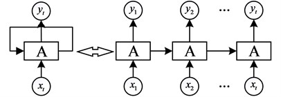
Sequence correlation is a very important feature of financial time series and it is indispensable when establishing prediction models. The Recurrent Neural Network (RNN) contains the historical information of the input time-series data, which can reflect the sequence-related features of the financial time series [27]. However, as shown in Fig.1, the output of a general recurrent neural network is only related to the current input. Regardless of past or future input, historical information of the time series or sequence-dependent features cannot be captured. Moreover, the circulatory neural network has the problem of gradient disappearance or gradient explosion, and can not effectively deal with the long-delayed time series, and thus the LSTM model is applied [28, 29].

Fig. 1General recurrent neural network structure

LSTM neural network is a new type of deep learning neural network, which is an improved structure of the recurrent neural network. LSTM solves the long-term dependence and gradient disappearance problems in the standard RNN by introducing the concept of a memory unit, ensuring that the model is fully trained, thereby improving the prediction accuracy of the model, and having a satisfactory effect in the processing of time series problems [30]. A standard LSTM network module structure is shown in Fig. 2.

Fig. 2Standard LSTM Neural Network module structure

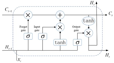
Each LSTM unit contains a unit of state C in time t, which can be considered as a memory unit. Each memory unit contains three “door” structures: forgotten doors, input doors, and output doors.

The first step: “forgetting the door”. According to the set conditions to determine which information in the memory unit needs to be forgotten, the gate reads $h_{t - 1}$ and $x_{t}$ and outputs a value between 0 and 1 to the cell state $C_{t - 1}$ . “1” indicates that all the information is retained, and “0” indicates that all information is discarded. The input of the “Forgetting Gate” consists of three vectors, namely the state $C_{t - 1}$ of the “memory cell” at the previous moment, the output $H_{t - 1}$ of the “memory cell” at the previous moment, and the input $X_{t}$ of the “memory cell” at the current moment. The weights, offsets, and output vectors of the “forgetting gate” sigmoid neural network layer are denoted by $W_{f}$ , $b_{f}$ and $f_{t}$ , respectively. The sigmoid activation function is shown in Eq. (22), and the output vector of the “forgetting gate” neural network layer is expressed as Eq. (23) shows:

22

σ (x) = \frac{1}{1 + e^{- x}},

23

f_{t} = σ (W_{f} • [h_{t - 1}, x_{t}] + b_{f}) .

The second step: “input door” determines which new information is added to the memory unit and updates the memory unit. The Sigmoid layer determines what information needs to be updated, $i_{t}$ is the hidden state at time $t$ , and a new candidate value vector ${\hat{C}}_{t}$ is created through $t a n h$ the network layer, and the updated memory cell state is $C_{t}$ , where $C_{t - 1}$ is the memory cell information of the previous moment:

24

\begin{array}{l} i_{t} = σ (W_{i} • [h_{t - 1}, x_{t}] + b_{i}), \\ {\hat{C}}_{t} = t a n h (W_{c} • [h_{t - 1}, x_{t}] + b_{c}), \\ C_{t} = f_{t} • C_{t - 1} + i_{t} • {\hat{C}}_{t} . \end{array}

The third step: the output gate, which determines the output of the network. First, the output part $O_{t}$ of the memory cell is determined by the Sigmoid layer, and then the memory cell state $C_{t}$ obtained in step 2 is processed by the tanh layer, and then it is multiplied by the output of the Sigmoid layer to obtain the output $h_{t}$ at that moment:

25

\begin{array}{l} O_{t} = σ (W_{O} • [h_{t - 1}, x_{t}] + b_{O}), \\ h_{t} = O_{t} • t a n h (C_{t}) . \end{array}

4.4. Evaluation criteria for predictive performance

In order to quantitatively evaluate the accuracy and stability of the proposed model, the root means squared error (RMSE), mean absolute error (MAE), mean absolute percentage error (MAPE), and coefficient of determination $R^{2}$ was used as evaluation criteria. These expressions are as follows:

26

R M S E = \sqrt{\frac{1}{N} \sum_{t = 1}^{N} (y_{t} - {\hat{y}}_{t})^{2}},

27

M A E = \frac{1}{N} \sum_{t = 1}^{N} |y_{t} - {\hat{y}}_{t}|,

28

M A P E = \frac{1}{N} \sum_{t = 1}^{N} |\frac{y_{t} - {\hat{y}}_{t}}{y_{t}}| \times 100 %,

29

R^{2} = 1 - \frac{\sum_{t} (y_{t} - {\hat{y}}_{t})^{2}}{\sum_{t} (y_{t} - {\bar{y}}_{t})^{2}} .

In the above equation, $y_{t}$ and ${\hat{y}}_{t}$ respectively represent the real value and predicted the value of time series at time $t$ , $\bar{y}$ is the mean value of time series, and $N$ is the length of time series. $R^{2}$ is the square of the correlation coefficient, and its value is generally between [0, 1]. The closer the value is to 1, the higher the fitting degree is, the better the prediction effect is.

5. Multi-model hybrid method prediction steps

The time-series data is decomposed into different sequence components by wavelet transform, then the chaotic characteristics of different sequences are judged, the Volterra model is established for the data with chaotic characteristics, the JGPC model is established for the sequences without chaotic characteristics, and then the above model is The predicted values are then subjected to the final predicted value estimation via the LSTM neural network. A multi-step prediction can be obtained according to the above form.

Fig. 3Model prediction structure diagram

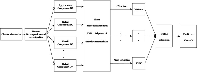
In this paper, a DWT and Volterra-JGPC-LSTM hybrid model is proposed to predict chaotic time series. The main implementation steps of the model are shown as follows and Fig. 3.

Step 1. Normalize the data to improve the convergence speed of the data during the training process. The Max-Min normalization method is used here, and the normalized sequence is $y_{t} = (y_{t} - y_{m i n}) / (y_{m a x} - y_{m i n})$ , where $y_{m a x}$ and $y_{m i n}$ are the maximum and minimum values in the sequence.

Step 2. Wavelet decomposition and single-branch reconstruction. Choosing the appropriate wavelet function and decomposition scale, multi-scale wavelet decomposition of chaotic time series, obtaining the approximate coefficients and detailed coefficients of the sequence, and then performing a single branch reconstruction on these coefficients to obtain a trend that can describe the trend of the original sequence. Low-frequency sequences and multiple high-frequency sequences that retain different information.

Step 3. Phase space reconstruction. The mutual information method is used to find the delay time, and the CAO method is used to calculate the embedded dimension t, and the low-frequency sequence and each high-frequency sequence are reconstructed in phase space, so as to form the corresponding training data and test data.

Step 4. Chaos characteristics of each sequence are distinguished through the correlation integral and Kolmogorov entropy.

Step 5. If the sequence has chaotic characteristics, the Volterra model is used for modeling prediction. If the sequence does not have chaotic characteristics, the JGPC model is used for modeling prediction.

Step 6. Finally, the prediction results of the above model are evaluated by the LSTM neural network, and obtain the final prediction results.

Step 7. The above Multi-model fusion method also has high accuracy for multi-step prediction. Its form can be described as follows:

(1) One-step prediction:

Calculate a one-step prediction $y (t + 1)$ based on the historical time series $\{y (1), y (2), \dots, y (t - 1), y (t)\}$ .

(2) Two-step prediction:

Calculate the two-step prediction value $y (t + 2)$ based on the historical time series $\{y (1), y (2), \dots, y (t - 1), y (t)\}$ and the one-step prediction value $y (t + 1)$ .

(3) Three-step prediction:

The three-step prediction value $y (t + 3)$ is calculated based on the historical time series $\{y (1), y (2), \dots, y (t - 1), y (t)\},$ the one-step prediction value $y (t + 1),$ and the two-step prediction value $y (t + 2)$ .

6. Data description

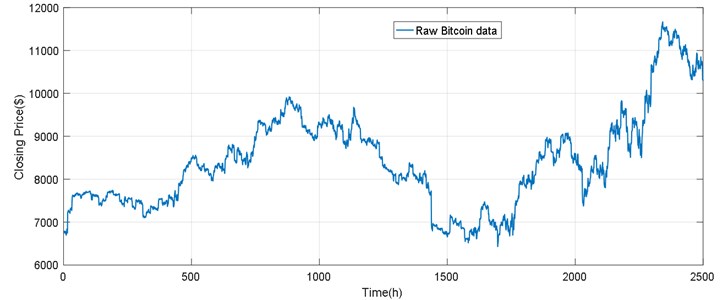
With the increase of Bitcoin application scenarios, its economic status has steadily increased and has attracted the attention of more investors [30]. Understanding the law of bitcoin price volatility, in order to correctly predict the trend of bitcoin trading, helping investors to rationally invest and avoid bitcoin price shocks in a timely manner is of great significance to promote the healthy and stable development of the bitcoin market [32]. Fig. 4 is a chart showing the Bitcoin market price, market value, and daily trading volume. In order to verify the validity of the algorithm proposed in this paper, we use the closing price of Bitcoin provided on https://coinmarketcap.com/ as the experimental data. The daily closing price data from April 28, 2013, to November 24, 2015, is used as a training set, and the daily closing price data from November 25, 2015, to March 23, 2016, is used as a test set. The experimental data used in this paper was bitcoin’s closing price per hour from 2017/6/1 17:00 to 2017/8/215:00:00, with a total of 1950 data points, as shown in Fig. 4.

Table 1The presentation of the two sets of datasets

Data		Number	Time
Bitcoin	Training set	1900	2017/6/1 17:00 — 2017/8/11 3:00:00
Bitcoin	Test set	100	2017/8/1 14:00:00—2017/8/21 5:00:00

The expression of the experimental data set is shown in Table 1. Experimental hardware conditions: Inter (R) Core (TM) i7-6700 CPU@3.40GHz, 16GB memory. The software environment: MATLAB2018a.

Fig. 4The raw Bitcoin data

7. Results and discussion

Daubechies wavelet of chaos and non-stationary time series has the very good features, adopting different $N$ values of DBN wavelet has the different treatment effect on the signal, in order to guarantee the real-time and accuracy, improve the generalization ability of forecasting model, and references according to the experiment, this paper use db6 wavelet transform was carried out on the experimental data decomposition reconstruction . Fig. 5 shows the result of the 6-layer decomposition and single reconstruction of bitcoin data using the db6 wavelet.

Fig. 5Wavelet decomposition of Bitcoin data

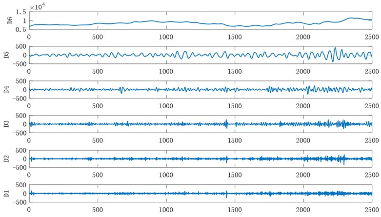
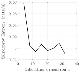
The time series of $d_{1}$ - $d_{5}$ and $a_{5}$ obtained by decomposition are judged by Kolmogorov entropy. The experimental results are shown in Fig. 6-Fig. 11 and Table 2. The entropy value of Kolmogorov of sequences $a_{5}$ and $d_{3}$ - $d_{5}$ is greater than 0. Therefore, the sequences of $a_{5}$ and $d_{3}$ - $d_{5}$ have chaotic characteristics. Kolmogorov entropy of $d_{1}$ and $d_{2}$ sequences is less than 0, so $d_{4}$ and $d_{5}$ sequences have non-chaotic characteristics.

Table 2The presentation of the two sets of datasets

Decomposition sequence	$a_{5}$	$d_{1}$	$d_{2}$	$d_{3}$	$d_{4}$	$d_{5}$
$K$ entropy	0.2514	–0.0224	–0.039	0.2717	0.4335	0.1896

Fig. 6a5 sequence K entropy

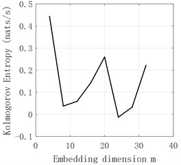
Fig. 7d1 sequence K entropy

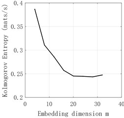
Fig. 8d2 sequence K entropy

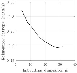
Fig. 9d3 sequence K entropy

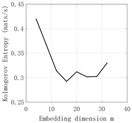
Fig. 10d4 sequence K entropy

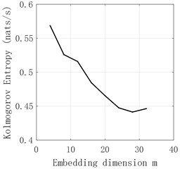
Fig. 11d5 sequence K entropy

8. Comparison of models

8.1. Set model parameters

This section validates the Bitcoin closing price prediction performance of the mixed Volterra-JGPC-LSTM model. The prediction process and model parameters are configured as follows, respectively establishing a Volterra model for sequences $a_{5}$ and $d_{3}$ - $d_{5}$ with chaotic characteristics, and establishing the JGPC model for sequences $d_{1}$ and $d_{2}$ without chaotic characteristics. The predicted values of these six sequences are then used as the input of the LSTM network for the final modeling prediction, so as to obtain the final predicted values. Firstly, the data is normalized to improve the convergence speed of the data in the training process. The Volterra model is modeled using a second-order truncation. The JGPC model with delay time $d =$ 4 was used for modeling. LSTM model training parameters are as follows: the target error, the learning rate is 0.01, the number of iterations is 10000, the size of input window is 6, the hidden layer is 1 in total, the number of hidden layer nodes is 40, and the output node is 1. The predicted results of $a_{5}$ and $d_{3}$ - $d_{5}$ are shown in Fig. 12 to Fig. 15, and the predicted results of $d_{1}$ - $d_{2}$ are shown in Fig. 16 to Fig. 17. The final predicted value of bitcoin closing price is obtained through the fusion prediction of the LSTM neural network, as shown in Fig. 18.

8.2. Results for Bitcoin data

In order to verify the prediction performance of the Volterra-JGPC-LSTM model for bitcoin closing price, a one-step, two-step, and three-step prediction performance experiment was conducted respectively with Volterra model, JGPC model, and LSTM model. In addition, to better compare the prediction model, set the same parameters in the model. For example, in the proposed model and comparison model, the input window size of the model is 20, and the range of test data is 100. The evaluation index of predictability uses RMSE, mean absolute error (MAE), mean absolute percentage error (MAPE) and determination coefficient $R^{2}$ , and calculates the percentage reduction and increase of $R^{2}$ in the Volterra-JGPC-LSTM model and comparison model mentioned in this paper. The comparison results of the prediction performance of each model are shown in Fig. 19 to Fig. 21 and Table 3.

Fig. 12a5 sequence Volterra model predicts the results

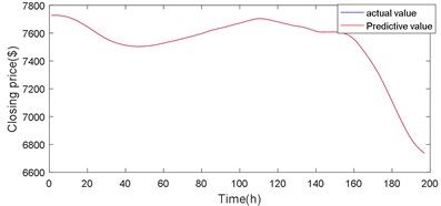
Fig. 13d5 sequence Volterra model predicts the results

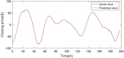
Fig. 14d4 sequence Volterra model predicts the results

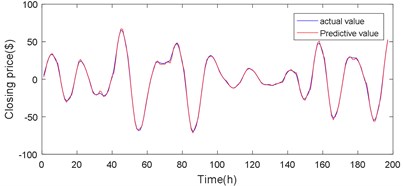
Fig. 15d3 sequence Volterra model predicts the results

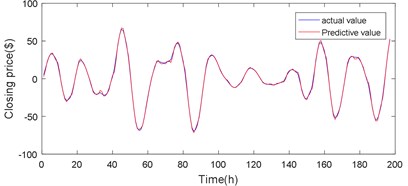
Fig. 16d2 sequence JGPC model predicts the results

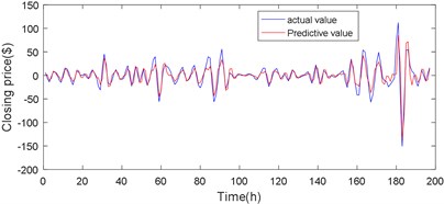
Fig. 17d1 sequence JGPC model predicts the results

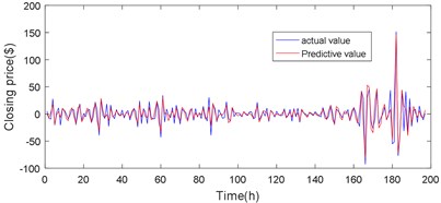
Table 3The evaluation results of different models for Bitcoin prediction

Forecasting models	Step	RMSE	MAE	MAPE	$R^{2}$
JGPC	1	135.7994	135.9089	0.0127	0.6118
	2	183.4745	137.5849	0.0257	0.7743
	3	206.0263	144.9206	0.0699	0.7221
Volterra	1	83.6344	76.3602	0.0071	0.8850
	2	112.5561	88.1330	0.0145	0.8689
	3	140.9246	96.2078	0.0256	0.8044
LSTM	1	57.3018	51.5189	0.0048	0.9464
	2	103.4552	71.9723	0.0104	0.8923
	3	125.3659	84.4987	0.0276	0.8281
Volterra-JGPC-LSTM	1	30.8011	23.8397	0.0022	0.9844
	2	96.5792	70.2331	0.0103	0.9145
	3	112.5689	99.0450	0.0315	0.8756

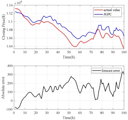
The forecast results are shown in Fig. 18, Fig. 19 and Table 3. The Volterra-JGPC-LSTM model presented in this paper has a significantly higher accuracy for the closing price prediction of Bitcoin than the JGPC model. Compared with the JGPC model in one-step, two-step, and three-step predictions, the RMSE of the Volterra-JGPC-LSTM model reduced by 27.45 %, 26.89 %, and 35.35 % respectively, and the MAE reduced by 29.55 %, 20.56 %, and 31.44 % respectively, MAPE reduced by 28.20 %, 26.39 %, and 19.55 % respectively, and $R^{2}$ increased by 3.24 %, 4.20 %, and 4.59 % respectively.

Fig. 18Volterra-JGPC-LSTM model prediction results

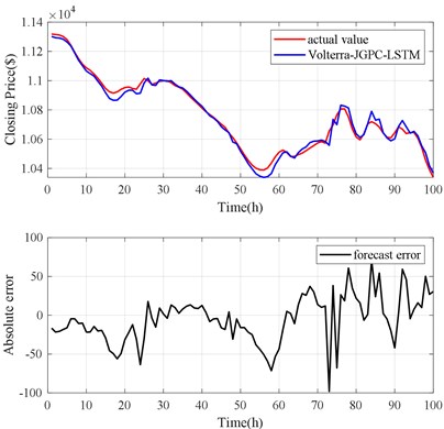
Fig. 19LSTM model prediction results

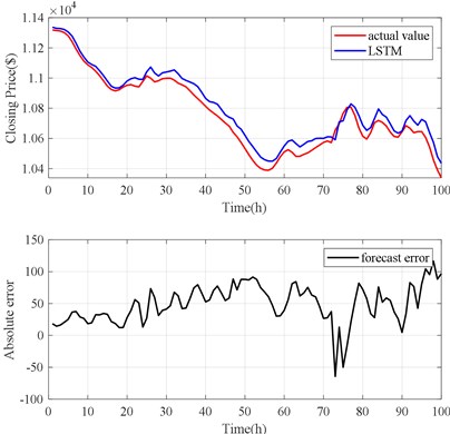
Fig. 20Volterra model prediction results

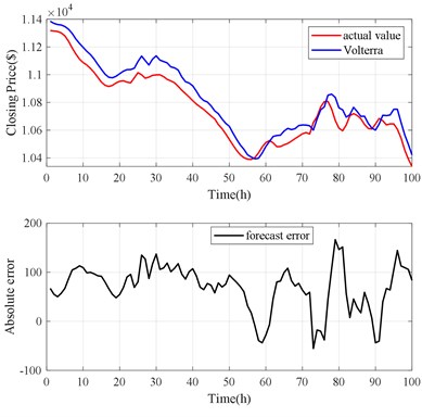
Fig. 21JGPC model prediction results

The forecast results are shown in Fig. 18, Fig. 20 and Table 3. The Volterra-JGPC-LSTM model presented in this paper has a significantly higher accuracy for the closing price prediction of Bitcoin than the Volterra model. Compared with the Volterra model in one-step, two-step, and three-step predictions, the RMSE of the Volterra-JGPC-LSTM model reduced by 20.33 %, 22.89 %, and 31.27 % respectively, and the MAE reduced by 31.21 %, 23.74 %, and 25.34 % respectively, MAPE reduced by 28.20 %, 26.39 %, and 19.55 % respectively, and $R_{2}$ increased by 3.24 %, 4.20 %, and 4.59 % respectively.

The forecast results are shown in Fig. 18, Fig. 21 and Table 3. The Volterra-JGPC-LSTM model presented in this paper has a significantly higher accuracy for the closing price prediction of Bitcoin than the LSTM model. Compared with the LSTM model in one-step, two-step, and three-step predictions, the RMSE of the Volterra-JGPC-LSTM model reduced by 22.53 %, 29.36 %, and 30.56 % respectively, and the MAE reduced by 25.225 %, 26.39 %, and 34.43 % respectively, MAPE reduced by 19.22 %, 29.39 %, and 18.56 % respectively, and $R^{2}$ increased by 3.24 %, 4.20 %, and 4.59 % respectively.

From the above experimental results, it can be seen that the DWT and Volterra-JGPC-LSTM hybrid model used in this paper has a significantly higher prediction accuracy for Bitcoin closing prices than other models.

9. Conclusions

In reality, chaotic time series are often affected by a variety of factors and are characterized by non-stationarity, non-linearity, and chaos. It is difficult for traditional single-model methods to make relatively accurate predictions for time series. In order to further improve the prediction accuracy, this paper will study time series pretreatment and depth algorithm and traditional algorithm, proposes a hybrid on the DWT and Volterra-JGPC-LSTM model to predict chaotic time series, using the proposed approach to the currency closing price modeling prediction, calculate the root mean square error (RMSE), mean absolute error (MAE), mean absolute percentage error (MAPE) and the determination coefficient $R^{2}$ of 82.2359, 57.9942, 0.0068, 0.9610, respectively. In order to verify the effectiveness of the mixed Volterra-JGPC-LSTM model algorithm proposed in this paper, the experimental results were compared with the JGPC model, LSTM model, and Volterra model respectively. The experimental results showed that a DWT and Volterra-JGPC-LSTM model proposed in this paper had significantly higher prediction accuracy of bitcoin closing price than other models. The method proposed in this paper has a wide application prospect and value for the prediction and analysis of the chaotic time series.

References

Corbet S., Meegan A., Larkin C., et al. Exploring the dynamic relationships between cryptocurrencies and other financial assets. Economics Letters, Vol. 165, 2018, p. 28-34.

Publisher
Satoshi Nakamoto Bitcoin: a Peer-To-Peer Electronic Cash System. Consulted, 2008.

Search CrossRef
Polasik M., Piotrowska A. I., Wisniewski T. P., Kotkowski R., Lightfoot G. Price fluctuations and the use of bitcoin: an empirical inquiry. International Journal of Electronic Commerce, Vol. 20, Issue 1, 2015, p. 9-49.

Publisher
Belke A., Setzer R. Contagion, herding and exchange-rate instabilitya survey. Intereconomics, Vol. 39, Issue 4, 2004, p. 222-228.

Publisher
Bri`ere M., Oosterlinck K., Szafarz A. Virtual currency, tangible return: Portfolio diversification with Bitcoins. Tangible Return: Portfolio Diversification with Bitcoins, 2013.

Publisher
Kaastra I., Boyd M. Designing a neural network for forecasting financial and economic time series Neurocomputing, Vol. 10, Issue 3, 1996, p. 215-236.

Publisher
Żbikowski K. Application of machine learning algorithms for bitcoin automated trading. Machine Intelligence and Big Data in Industry, Springer International Publishing, 2016.

Publisher
Zhang Zhaxi, Che Wang Spatiotemporal variation trends of satellite-based aerosol optical depth in China during 1980-2008. Atmospheric Environment, Vol. 45, Issue 37, 2011, p. 6802-6811.

Publisher
Cao L. Practical method for determining the minimum embedding dimension of a scalar time series. Physica D, Vol. 110, Issues 1-2, 1997, p. 43-50.

Publisher
Shu Yong L., Shi Jian Z., Xiang Y. U. Determinating the embedding dimension in phase space reconstruction. Journal of Harbin Engineering University, 2008.

Search CrossRef
Jiang Y., Zhang B., Xing F., et al. Super-short-term multi-step prediction of wind power based on GA-VNN model of chaotic time series. Power System Technology, 2015.

Search CrossRef
Murguia J. S., Campos Cantón E. Wavelet analysis of chaotic time series. Revista Mexicana De Física, Vol. 52, Issue 2, 2006, p. 155-162.

Search CrossRef
Ciocoiu Iulian B. Chaotic Time Series Prediction Using Wavelet Decomposition. Technical University Iasi, 1995.

Search CrossRef
Zhongda Tian, et al. A prediction method based on wavelet transform and multiple models fusion for chaotic time series. Chaos, Solitons and Fractals, Vol. 98, 2017, p. 158-172.

Publisher
Xu L., Tao G. Independent component analyses, wavelets, unsupervised nano-biomimetic sensors, and neural networks V. Proceedings of SPIE – The International Society for Optical Engineering, 2007.

Search CrossRef
Khashei M., Bijari M., Ardali G. A. R. Improvement of auto-regressive integrated moving average models using fuzzy logic and artificial neural networks (ANNs). Neurocomputing, Vol. 72, Issue 4, 2009, p. 956-967.

Publisher
Zhou H. C., Peng Y., Liang G. H. The research of monthly discharge predictor-corrector model based on wavelet decomposition. Water Resources Management, Vol. 22, Issue 2, 2008, p. 217-227.

Publisher
Mallat S. G. Multiresolution Representations and Wavelets. University of Pennsylvania, 1988.

Search CrossRef
Chawla N. V., Bowyer K. W., Hall L. O., et al. SMOTE: Syntheticminority over-sampling technique. Journal of Artificial Intelligence Research, Vol. 16, Issue 1, 2002, p. 321-357.

Publisher
Cheng J., Yu D., Yu Y. The application of energy operator demodulation approach based on EMD in machinery fault diagnosis. Mechanical Systems and Signal Processing, Vol. 21, Issue 2, 2007, p. 668-677.

Publisher
Omer F. D. A hybrid neural network and ARIMA model for water quality time series prediction. Engineering Applications of Artificial Intelligence, Vol. 23, Issue 4, 2010, p. 586-594.

Publisher
Lukoševičius Mantas, Jaeger H. Reservoir computing approaches to recurrent neural network training. Computer Science Review, Vol. 3, Issue 3, 2009, p. 127-149.

Publisher
Wang G. F., Li Y. B., Luo Z. G. Fault classification of rolling bearing based on reconstructed phase space and Gaussian mixture model. Journal of Sound and Vibration, Vol. 323, Issues 3-5, 2009, p. 1077-1089.

Publisher
Wang Pingli, Song Bin, Wang Ling Application of Kolmogorov entropy for chaotic time series. Computer Engineering and Applications, Vol. 42, Issue 21, 2006.

Search CrossRef
Zhao Guibing, Shi Yanfu simultaneous calculation of correlation dimensions and Kolmogorov entropy from chaotic time series. Chinese Journal of Computational Physics, Vol. 3, 1999, p. 309-315.

Search CrossRef
Li Y., Zhang Y., Jing W., et al. The Volterra adaptive prediction method based on matrix decomposition. Journal of Interdisciplinary Mathematics, Vol. 19, Issue 2, 2016, p. 363-377.

Publisher
Kong W., Dong Z. Y., Jia Y., et al. Short-term residential load forecasting based on LSTM recurrent neural network. IEEE Transactions on Smart Grid, Vol. 10, Issue 1, 2019, p. 841-851.

Publisher
Gers Felix A., Jürgen Schmidhuber, Fred A. Cummins learning to forget: continual prediction with LSTM. Neural Computation, Vol. 12, Issue 10, 2000, p. 2451-2471.

Publisher
Kim S., Kang M. Financial series prediction using Attention LSTM. Papers, 2019.

Search CrossRef
Cortez B., Carrera B., Kim Y. J., et al. An architecture for emergency event prediction using LSTM recurrent neural networks. Expert Systems with Applications, Vol. 97, 2018, p. 315-324.

Publisher
Kristoufek L. What are the main drivers of the Bitcoin price? evidence from wavelet coherence analysis. PloS one, Vol. 10, Issue 4, 2015, p. 0123923.

Publisher
Matevž Pustišek, Andrej Kos Approaches to front-end IoT application development for the ethereum blockchain. Procedia Computer Science, Vol. 129, 2018, p. 410-419.

Publisher

Cited by

A High-Precision Chaotic LSTM Network Model Optimized by FrVMD for the Earth Natural Pulse Electromagnetic Signal Intensity Trend Forecast

(2024)

Multilayer Perceptron Network Optimization for Chaotic Time Series Modeling

Mu Qiao | Yanchun Liang | Adriano Tavares | Xiaohu Shi

(2023)

Proceedings of the 2023 4th International Conference on Computing, Networks and Internet of Things

Zhao Wang

(2023)

Kolmogorovʼ entropy to investigate variation of forest soil properties in the Czech Republic

Pavel Samec

(2022)

On the Prediction of Chaotic Time Series using Neural Networks

Josue Alexis MARTİNEZ-GARCİA | Astrid Maritza GONZALEZ-ZAPATA | Ericka Janet RECHY-RAMİREZ | Esteban TLELO-CUAUTLE

(2022)

High precision reconstruction of silicon photonics chaos with stacked CNN-LSTM neural networks

(2022)

Modelling, Simulation and Applications of Complex Systems

Noor A. Ahmad | Shazia Javed

(2021)

Time series analysis and prediction of nonlinear systems with ensemble learning framework applied to deep learning neural networks

Shao-Chun Wen | Cheng-Hsiung Yang

(2021)

A Novel Error Correction Approach to Improve Standard Point Positioning of Integrated BDS/GPS

Luyao Du | Jing Ji | Zhonghui Pei | Wei Chen

(2020)

About this article

Received

06 February 2019

Accepted

17 July 2019

Published

15 November 2019

SUBJECTS

Chaos, nonlinear dynamics and applications

DOI

https://doi.org/10.21595/jve.2019.20579

Keywords

phase space reconstruction; Multi-model hybrid; chaos characteristics; Volterra-JGPC-LSTM model

Acknowledgements

The work in this paper was supported by the National Natural Science Foundation of China under Grant No. (61001174); Tianjin Science and Technology Support and Tianjin Natural Science Foundation of China under Grant No. (13JCYBJC17700).

This is an open access article distributed under the Creative Commons Attribution License, which permits unrestricted use, distribution, and reproduction in any medium, provided the original work is properly cited.

Previous article in issue Previous Next article in issue Next

Research article

2021 01 09

Vibration performance prediction and reliability analysis for rolling bearing

Fannian Meng, Xiaoyun Gong, Wenliao Du, Liangwen Wang, Feng Zhao, Liwei Li

Research article

2018 09 30

Local Volterra multivariable chaotic time series multi-step prediction based on phase points clustering

Feng Han, Shuying Yang, Shibao Song

Research article

2018 02 15

Research and application of Volterra series theory in rolling bearing fault state feature extraction

Haitao Wang, Zhenya Kang, Lichen Shi, Kun Wang, Xiao Zhang

Research article

2018 02 15

Structural state inspection using dual-tree quaternion wavelet transform

Tongqun Ren, Meiling Hui, Xiaodong Wang, Zhiyong Zhang, Junsheng Liang

T. Feng, S. Yang, and F. Han, “Chaotic time series prediction using wavelet transform and multi-model hybrid method,” Journal of Vibroengineering, Vol. 21, No. 7, pp. 1983–1999, Nov. 2019, https://doi.org/10.21595/jve.2019.20579

Copy Extrica

Copied to clipboard!

TY  - JOUR
DO  - 10.21595/jve.2019.20579
UR  - https://doi.org/10.21595/jve.2019.20579
TI  - Chaotic time series prediction using wavelet transform and multi-model hybrid method
T2  - Journal of Vibroengineering
AU  - Feng, Tian
AU  - Yang, Shuying
AU  - Han, Feng
PY  - 2019
DA  - 2019/11/15
PB  - JVE International Ltd.
SP  - 1983-1999
IS  - 7
VL  - 21
SN  - 1392-8716
SN  - 2538-8460
ER  - 

Copy Ris

Copied to clipboard!

@article{Feng_2019,
	doi = {10.21595/jve.2019.20579},
	url = {https://doi.org/10.21595/jve.2019.20579},
	year = 2019,
	month = {nov},
	publisher = {{JVE} International Ltd.},
	volume = {21},
	number = {7},
	pages = {1983--1999},
	author = {Tian Feng and Shuying Yang and Feng Han},
	title = {Chaotic time series prediction using wavelet transform and multi-model hybrid method},
	journal = {Journal of Vibroengineering}
}

Copy Bibtex

Copied to clipboard!

[1]T. Feng, S. Yang, and F. Han, “Chaotic time series prediction using wavelet transform and multi-model hybrid method,” Journal of Vibroengineering, vol. 21, no. 7, pp. 1983–1999, Nov. 2019, doi: 10.21595/jve.2019.20579.

Copy IEEE

Copied to clipboard!

Feng, Tian, Shuying Yang, and Feng Han. “Chaotic Time Series Prediction Using Wavelet Transform and Multi-Model Hybrid Method.” Journal of Vibroengineering 21, no. 7 (November 15, 2019): 1983–99. https://doi.org/10.21595/jve.2019.20579.

Copy Chicago

Copied to clipboard!

Chaotic time series prediction using wavelet transform and multi-model hybrid method

Abstract

1. Introduction

2. Chaotic time series decomposition based on Mallat discrete wavelet transform

3. Judgment of chaotic characteristics

3.1. Phase space reconstruction

3.2. Judging the chaotic characteristics of Kolmogorov entropy

4. Multi-model fusion method based on Volterra-JGPC-LSTM

4.1. An improved generalized predictive control model (JGPC)

4.2. Volterra chaotic time series adaptive prediction model

4.3. Long short-term memory (LSTM)

4.4. Evaluation criteria for predictive performance

5. Multi-model hybrid method prediction steps

6. Data description

7. Results and discussion

8. Comparison of models

8.1. Set model parameters

8.2. Results for Bitcoin data

9. Conclusions

References

Cited by

About this article

Related Articles