Abstract
This publication provides a discussion concerning research aimed to analyse running properties of PRT vehicles. A PRT vehicle is guideway vehicle equipped with rubber-tyred wheels, running on a flat subgrade guideway of special design. The guideway cross-section is similar to that of a C-shaped beam with two outer limiting edges. This specific design characteristic of the running system of PRT vehicles distinguishes them from typical rail vehicles, where the latter can move along the track by the action of a unit referred to as the centring mechanism, operating at the contact of profiled wheels with the running rail head. In a PRT vehicle, the typical railway centring mechanism has been removed and substituted with a system of outer and inner rollers, forming what is referred to as a passive switch system, responsible for carrying the vehicle along the guideway and within the boundaries delimited by its edges by the action of the rollers’ contact forces. Compared to railway infrastructure, this system is characterised by different dynamic properties, and it has not been sufficiently researched yet. The goal of this article is to analyse motion stability of a PRT vehicle with a passive switch system and having the following structural features: wheel sets with beams turning against the vehicle body and independently revolving wheels, non-turning rubber-tyred and non-profiled wheels rolling on a flat surface, and a set of outer and inner rollers performing the passive switch system’s functions. The paper describes a PRT vehicle simulation model. It has been assumed that the model’s design and parameters describe a scaled vehicle/guideway system whose physical model is actually set at a laboratory testing station on premises of the Warsaw University of Technology. The article provides results of simulation studies of motion stability pertaining to the following characteristics: radial positioning, yawing, sticking to the guideway edge, self-excited vibrations of wheel sets as well as free vibrations. It also discusses results of an analysis of sensitivity of the model’s parameters against selected control parameters (model’s design parameters) and assessment indicators which describe the intensity of the yaw type torsional vibrations of wheel sets. The article closes with a discussion on the potential to use the results of the tests conducted under the study on the scaled vehicles in question for purposes of vehicles of real-life dimensions.
1. Introduction
In light of the Polish state government’s recent electro-mobility programme officially referred to as “Elektro-Mobilność”, an actual opportunity has emerged to implement a Personal Rapid Transit (PRT) system in Poland. It should be noted that the PRT system belongs to a specific category of guideway transport systems known as ATN (Automated Transit Network). This transport mode is intended to carry passengers between specific points without halting at intermediate stops by means of small and fully automatic electric vehicles running in separate guideways. It is for the specificity of this public transport mode that it cannot be considered massive transport in nature, but it complements the latter very effectively. There are four PRT systems currently in operation around the world:
• System delivered by the Dutch company 2getthere, commissioned in 2010 in Masdar City, Abu Dhabi [1],
• System delivered by the British company ULTra PRT, commissioned in 2011 at terminal no. 5 of London Heathrow Airport [2],
• System delivered by the Korean-Swedish consortium of Vectus, commissioned in 2013 in the Suncheon national part in South Korea [3, 4].
Mexican ModuTram system launched in 2014 at the WTC Morelos Convention Centre in Mexico [5].
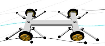
Fig. 1Scaled physical model of a PRT vehicle at a laboratory testing station [30]
![Scaled physical model of a PRT vehicle at a laboratory testing station [30]](https://static-01.extrica.com/articles/20577/20577-img1.jpg)
The PRT transport system is a subject which has already been addressed in numerous publications. “At the beginning, initial concepts of automatic transport were presented [6, 7], and relationships between the political milieu and technological innovations were analysed [8]. Many papers published in subsequent years concerned specific research problems and implementations [9-12]. The literature was also rich in articles addressing the general approach to automatic means of transport considered as innovative means of urban transport [13] or as means of transport intended to be deployed within a specific limited area [14-16]. The report prepared at the Mineta Transportation Institute [17] may be regarded as a resume of the then state of research and technology in the field of automatic transport (ATN) worldwide. Authors of the report also presented their perspective of future developments in this mode of transport” [18]. Part of the scientific literature addressing this body of problems focuses on the matters of vehicle traffic control and management, safety and flow capacity analysis, as considered in papers [19, 20], [21-23].
With regard to the Polish research in the sphere of the PRT transport, the most popular solution was conceived under the “ECO-Mobilność” research project implemented in the years 2009-2015 at the Warsaw University of Technology [24, 25]. However, it should be noted that the project goal never was to deploy a specific system, but only to perform scientific and research activity. In the part pertaining to PRT, the project’s results were discussed in papers [26, 27]. A physical model of a vehicle/guideway/control system setup was developed to a scale of 1:4 along with a 1:1 physical model of the vehicle cabin, and a unique PRT network simulator was created. The Faculty of Electrical Engineering and the Faculty of Transport of the Warsaw University of Technology built two laboratory testing stations to run experimental tests of a PRT system in a scale of 1:4. The most recent publications include papers addressing the problems of traffic control [28], dimensioning of a contactless power supply system for PRT units [29, 30, 18], or a linear induction motor design intended for PRT [31].
2. Scope and purpose of the study
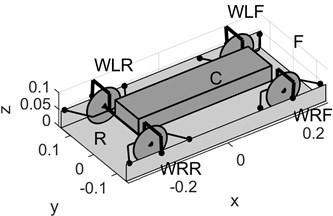
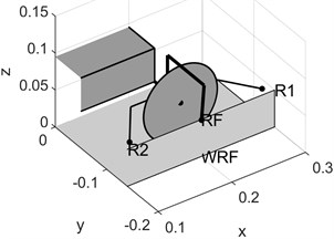
This article presents results of the latest studies conducted for the sake of analysis of motion stability of PRT vehicles running in branched guideway systems featuring switches. The studies on the problem of motion stability of PRT vehicles performed to date pertained to non-branched guideway sections, and the author took part in them. Papers [27] and [26] provide results of studies on the properties of travel in straight or curved sections (with a fixed turning radius) covered at a constant speed. The vehicle and guideway model currently being developed differs from the previous one in that its design stems from the structure of the physical model at hand. The model’s design has been schematically illustrated in Fig. 2: a) overview, b) right wheel’s set of passive switch rollers. The model is characterised by the following structural features (components): wheel sets with beams turning against the vehicle body and independently rotating wheels, non-turning rubber-tyred and non-profiled wheels rolling on a flat surface, and a set of outer and inner rollers performing the passive switch system’s functions. Moreover, the model’s parameters correspond to the physical model’s design parameters. Fig. 3 depicts the scaled vehicle model’s running conditions: a) the laboratory guideway fragment of an inter-station section between the START and STOP stations selected for purposes of the analysis, b) velocity profile. The thick solid lines shown in Fig. 3(a) represent the sides (edges) of the guideway fragment used. The thin broken line marks the guideway axis and the lateral branches of the guideway sections not used in the run. Fig. 3b shows the speed curve of a strenuous cycle completed in the selected inter-station section, as determined by taking into account the limitations to the drive system’s operating conditions [30].
Fig. 2Model’s arrangement of solid bodies: a) overview, b) right wheel’s set of passive switch rollers. Designations: WLF WRF WLR WRR – wheels: left front, right front, left rear, right rear, F and R – front and rear wheel set, R1 and R2 – inner rollers, RF – outer roller
a)
b)
Fig. 3PRT model’s running conditions: a) laboratory guideway fragment used for the trial run, b) velocity profile [30]. Designations: START – initial station, STOP – terminal station. Beginning and end points of switches: P1 – beginning of switch 1, P11 – end of switch 1, P2 and P21 – beginning and end of switch 2, P3 and P31 – beginning and end of switch 3
![PRT model’s running conditions: a) laboratory guideway fragment used for the trial run, b) velocity profile [30]. Designations: START – initial station, STOP – terminal station. Beginning and end points of switches: P1 – beginning of switch 1, P11 – end of switch 1, P2 and P21 – beginning and end of switch 2, P3 and P31 – beginning and end of switch 3](https://static-01.extrica.com/articles/20577/20577-img4.jpg)
a)
![PRT model’s running conditions: a) laboratory guideway fragment used for the trial run, b) velocity profile [30]. Designations: START – initial station, STOP – terminal station. Beginning and end points of switches: P1 – beginning of switch 1, P11 – end of switch 1, P2 and P21 – beginning and end of switch 2, P3 and P31 – beginning and end of switch 3](https://static-01.extrica.com/articles/20577/20577-img5.jpg)
b)
The purpose of the study is to analyse the motion stability of the vehicle model in the test guideway (featuring straight and curved sections as well as switches) for the running conditions defined under the planned experiment, i.e. from the START station to the STOP station, assuming the velocity profile illustrated in Fig. 3(b). The studies performed by the computer simulation method will serve the purpose of analyses of the following motion characteristics: radial positioning, yawing, sticking to the guideway edge, self-excited vibrations of wheel sets as well as free vibrations. What will also be proposed is specific assessment indicators describing the intensity of the yaw type torsional vibrations of wheel sets. The paper will provide results of the model parameter sensitivity analysis against selected control parameters (model’s design parameters) as well as the assessment indicators proposed.
At this point, it should be noted that the most serious problem facing the author in the studies in question is certainly the assessment of their reliability and utility value. It boils down to the fact that there is virtually no PRT test guideway section in Poland where full-scale tests of vehicles can be performed. And no such facility will be built in the foreseeable future. In other words, it is impossible to validate a model of real-life dimensions. Consequently, the only way to study the running properties of PRT vehicles remains to be testing of scaled models. Scaled testing is a common method used in different types of research, including to study navigability of ship models. The literature of the subject also mentions cases where this method was used to study rail vehicles [32].
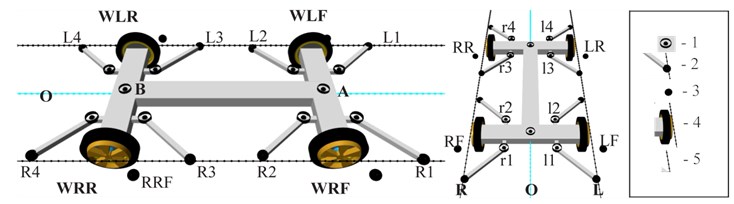
Fig. 4Nominal vehicle model: side view and front view. Designations: 1 – kingpins, 2 – inner rollers, 3 – outer rollers, 4 – rubber-tyred wheels, 5 – guideway sides (edges), WLF – left front wheel, WRF – right front wheel, WLR – left rear wheel, WRR – right rear wheel, A – front wheel set kingpin, B – rear wheel set kingpin, R1 R2 R3 R4 – right inner rollers, L1 L2 L3 L4 – left inner rollers, RF RR – right outer rollers, LF LR – left outer rollers, r1 r2 r3 r4 – kingpins of right roller arms, l1 l2 l3 l4 – kingpins of left roller arms
3. MBS (Multibody Dynamic System) model of the vehicle system
The simulation model of the vehicle/guideway system has been developed in the Matlab-Simulink_Simscape (Multibody) environment. The rubber-tyred wheel model has been described using library mf – tyre TNO Delft Tyre [33]. Fig. 4 provides a visualisation of the nominal vehicle model in side view and front view.
The model is composed of three fundamental solid bodies (body C) and two-wheel set axles (R and F) (Fig. 2(a)). The bodies are connected via kingpins marked in Fig. 4 as A and B. The additional elements are support brackets for the rollers and the wheel. The roller support brackets are connected with axles via kingpins.
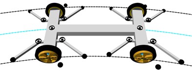
Fig. 5 illustrates main vehicle running modes: a) two-edge guideway, b) one-edge guideway at a switch. The vehicle basically runs in a two-edge guideway (Fig. 5(b)). This is the case where the vehicle is only guided by the system of inner rollers. The outer rollers are always lowered on one side of the vehicle, while they are raised on the other side; however, under normal operating conditions in a two-edge guideway, the outer rollers never contact the guideway’s outer edge. The vehicle’s outer rollers contact the guideway edge when it is running in a one-edge guideway, i.e. at switches. Where this is the case, they are decisive of the vehicle motion direction (Fig. 5(b)).
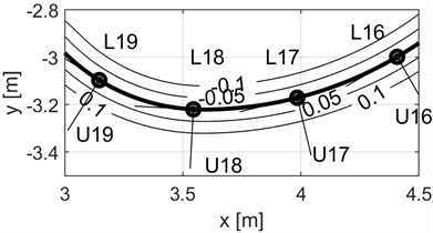
Contact forces of the rollers are determined with reference to the distance between the roller and the guideway edge. In order to establish these distances, one needs an adequate computational model, which bears the working name of “guideway edge” in this study. The guideway edge model has been visualised as shown in Fig. 6. The figure represents the model as isolines of distance from the guideway edge line. The thick line (isoline “0”) corresponds to the guideway edge. In this case, the contact forces of inner rollers are generated for positive distance values (on the left-hand side of the coordinate systems), while those of outer rollers – for negative values (on the right-hand side). In the simulation model, the guideway edge model is represented as an interpolation function enabling the distance value to be determined at each point of the guideway:
where: – distance in the normal direction, – guideway edge model’s interpolation function, and – coordinates in the Cartesian reference system.
Fig. 5Basic running modes: a) in two-edge guideway, b) in one-edge guideway, at switch
a)
b)
Fig. 6Guideway edge model (fragment). Designations: L16, L17, L18, L19 – points distributed at regular intervals along the guideway edge (every 0.5 m in the figure); U16, U17, U18, U19 – systems of coordinates of the guideway edge lines at selected points; 0.1, 0.05, 0, –0.05, –0.1 – isolines of distance (lines of fixed distance) from the guideway edge
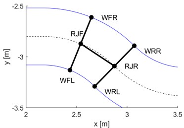
The forces generated in the rollers induce the turn of wheel sets. Fig. 7 illustrates two possible variants of positioning of the wheel sets against the guideway: a) radial, b) non-radial. The distinguishing feature of the radial positioning (Fig. 7(a)) is that the axis of wheel sets is arranged along the normal directions. Where this is the case, the vehicle axis beginning and end points (points of kingpins A and B, as in Fig. 4) should be aligned with the guideway axis. In practice, the vehicle is hardly ever positioned in this manner.
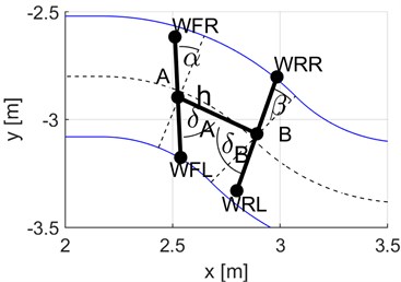
Fig. 7Vehicle positioning variants: a) radial (reference), b) non-radial (yaw values higher than actually). Designations of the parameters determined: δA, δB – turning angles of wheel sets, α, β – yaw angles of wheel set axes
a)
b)
However, this positioning is often used as the reference positioning to describe the yaws in the actual positioning of the vehicle’s solid bodies in the guideway. The yaws assumed for the sake of this study have been defined in Fig. 7(b). The designations used are as follows: , – turning angles of wheel sets, , – yaw angles of wheel set axes, – distance from guideway axis.
4. Study of running properties
PRT vehicles are guided along the guideway by a system known as a passive switch, composed of outer and inner rollers (Fig. 2(b)). The object of the simulation tests should be to study the following running properties:
• Radial positioning,
• Yawing,
• Sticking (to the guideway edge),
• Self-excited vibrations of wheel sets, and free vibrations.
Torsional vibrations of the front axis may occur while the vehicle is running in both straight and curved sections. The points where the system is particularly exposed to this type of vibrations are switches. The vibration excitation mechanism has been shown in Fig. 8.
Bearing the purpose of the study in mind, namely to analyse the running properties of PRT vehicles in branched guideways, the research objective is to analyse sensitivity of the model’s parameters. On account of the model design as well as the guideway model, the scope of sensitivity testing may comprise the following structural parameters:
• Guideway geometry parameters (normal two-edged, special one-edged, branched with switches, straight, curved),
• Parameters of generators of the tyre model’s longitudinal and lateral forces (considering the possibility to use different structural materials for wheels and the substrate),
• Parameters of roller arms (considering the possibility to change the values of torsional elasticity, torsional damping and arm length),
• Parameters of the axle kingpin for running wheels (torsional elasticity and damping),
• Parameters of clearance between the roller and the guideway edge (roller-to-guideway edge distance).
Fig. 8Visualisation of the front wheel set axle positioning while running onto a switch, showing the mechanism for generation of front axle torsional vibrations: a), b), c), d) – phases of motion. Designations: – roller’s reactive force, – torque of kingpin A
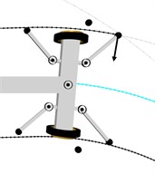
a)
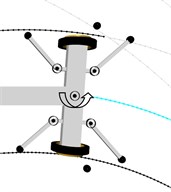
b)
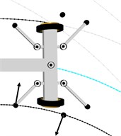
c)
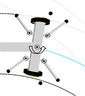
d)
5. Nominal parameters of a scaled vehicle/guideway model
The nominal parameters of the vehicle model (calculated as assumed in the design) have been collated in Table 1.
Preliminary analyses of results of the simulation tests have revealed that the intensity of torsional vibrations of wheel set axles mainly depends on the parameters of torsional elasticity and damping in kingpins (A and B – Fig. 4) as well as on the stiffness and lateral damping of wheel tyre treads. Further on in the study, it is assumed that these parameters perform the function of what is referred to as control variables of the model parameter sensitivity analysis.
Table 1Vehicle model’s nominal parameters
Element | Element designation in Fig. 2, 3, 4 | Element’s parameters | Unit of measure | Value |
Guideway | (Fig. 3) | Width | m | 0.3 |
Vehicle body | C (Fig. 2) | Length, width, height | m | [0.3, 0.18, 0.075] |
Wheel set axle | R, F (Fig. 2) | Length, width, height | m | [0.05, 0.14, 0.05] |
Front rollers’ arms | z1 (Fig. 2) | Length, width, height | m | [0.1294, 0.01, 0.01] |
Rear rollers’ arms | z2 (Fig. 2) | Length, width, height | m | [0.1176, 0.01, 0.01] |
Inner roller’s arm | W (Fig. 2) | Arm length, displacement against wheel axis | m | [0.05, 0.05] |
Axle kingpin for front wheels | A (Fig. 4) | Torsional elasticity and damping [, ] | N·m/deg, N·m/(deg/s) | [0.25, 0.01] |
Axle kingpin for rear wheels | B (Fig. 4) | Torsional elasticity and damping [, ] | N·m/deg, N·m/(deg/s) | [0.1, 0.01] |
Roller arm kingpin | r1–r4 & l1–l4 (Fig. 2, Fig. 4) | Torsional elasticity and damping [, ] | N·m/deg, N·m/(deg/s) | [2.5, 0.05] |
Wheel rim inertia | WLF, WRF, WLR, WRR (Fig. 2, Fig. 4) | Mass, inertia , inertia | kg, kg·m2 | [0.641, 0.0009, 0.0005] |
Tyre dimension | – | Radius, width, rim radius | m | [0.05, 0.02, 0.05] |
Tyre inertia | – | Mass, inertia , inertia | kg, kg·m2 | [0.05, 3.11e-5,1.18e-4] |
Tyre stiffness | – | Vertical stiffness, damping | N/m, N/(m/s) | [1,850,000, 5,000] |
In the TNO Delft Tyre model, the lateral force is determined by application of what is commonly referred to as the Magic Formula. According to this formula, the lateral force scaling is performed using the lateral friction coefficient (marked as in this paper). For the sake of the studies in question, it has been assumed that the range of change to this coefficient is 0.1–1.2. The manner in which the value of the coefficient of torsional elasticity and torsional damping changes in axle kingpins for wheel sets (A and B – Fig. 4) can be similarly described by defining an adequate scale factor:
where: , – nominal values of torsional elasticity and torsional damping in kingpin A or B, as provided in Table 1, , – values modified by application of the scale factor, – scale factor (coefficient of torsional elasticity and torsional damping). What has been assumed for the model parameter sensitivity analyses is that the variability range of this coefficient is 0.5–2.0 [–].
6. Simulation results
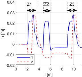
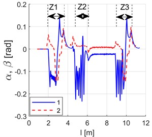
Fig. 9 shows turning angle curves for the front () and the rear () wheel set (for angle designations, see Fig. 7(b)) derived as results of the simulation of dynamics of the model whose parameters have been summarised in Table 1. Fig. 10 provides curves of yaw angles of wheel axles against the radial direction, i.e. curves of quantities , (Fig. 7(b)). Fig. 11 shows curves of distance between wheel axle centre points and the guideway axis, designated in Fig. 7(b) as . The above curves imply that the vehicle does not position itself radially (on radial positioning, the aforementioned characteristics would assume the value of zero).
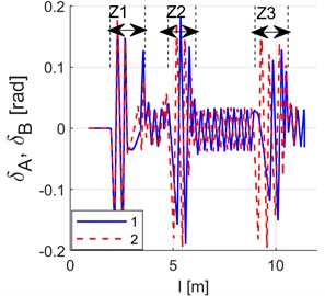
In the periods of time when the vehicle travels at switches, one can observe varying components of a decaying nature in the curves of the front axle’s turning and yaw angles. The vibration mechanism has been explained in Fig. 8. The vibration decay is linked with a relatively high value of wheel grip. Particularly high values of the front axle’s yaw angles against the radial direction can be witnessed when the vehicle is running onto a switch. This property is a consequence of the guideway design assuming that there is clearance between rollers and the guideway edge. Having entered the switch zone, not until the outer roller covers a short distance which eliminates the clearance resulting from the vehicle’s original positioning can it contact the guideway edge. Over this time, even though the vehicle is running in a curved trajectory, its wheel axles cannot position themselves radially due to absence of the roller guiding force.
Fig. 9Simulation results. Axle turning angles for: 1 – front wheels δA, 2 – rear wheels δB. Route sections at switches: Z1 – switch 1, Z2 – switch 2, Z3 – switch 3

Fig. 10Simulation results. Yaw angles of wheel axles against radial direction: 1 – front axle α, 2 – rear axle β. Route sections at switches: Z1 – switch 1, Z2 – switch 2, Z3 – switch 3
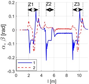
Fig. 11Simulation results. Curves of distance between wheel axle centre points and guideway axis: 1 – front axle, 2 – rear axle. Route sections at switches: Z1 – switch 1, Z2 – switch 2, Z3 – switch 3
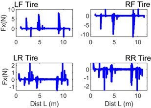
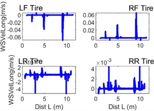
What matters greatly to the model’s motion characteristics is the wheel tyre tread model. Fig. 12 provides graphs of longitudinal force and longitudinal wheel slip velocity, while Fig. 13 the corresponding lateral quantities. What both Figs. 12 and 13 show is the considerable increases in the force and slip values while the vehicle is passing switches.
Fig. 12Selected instantaneous curves of quantities characterising the contact between the wheel tyre tread and the guideway surface: a) Fx – longitudinal force, b) WSVelLong – longitudinal wheel slip velocity
a)
b)
Fig. 13Selected instantaneous curves of quantities characterising the contact between the wheel tyre tread and the guideway surface: a) Fy – lateral force, b) WSVelLat – lateral wheel slip velocity
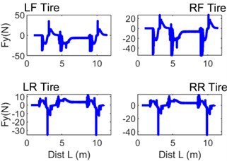
a)
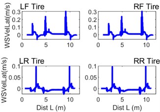
b)
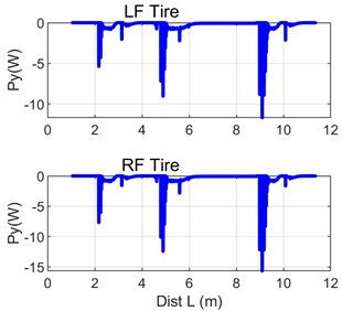
Moreover, one can notice that the characteristic values of lateral grip are significantly higher than those of the corresponding longitudinal quantities. Fig. 14 illustrates the instantaneous power loss in front wheels on account of the action of lateral forces and displacements.
Fig. 14Curves of instantaneous power of lateral motion of front rubber-tyred wheels
7. Characteristics of torsional vibration curves of wheel sets
In the case addressed in this paper, the purpose of the parameter sensitivity analysis is to explain the impact of specific structural parameters on the properties of torsional vibrations of the vehicle’s wheel set axles which the simulation results evidence (particularly in the periods when the vehicle is passing switches). The effect exerted by changing properties of the vibrations may be showcased by adequately changing the values of the assumed model simulation parameters.
Fig. 15 shows curves of yaw angles of wheel set axles against the radial direction which describe the results of the model simulation with modified scale parameters of lateral tread grip and torsional elasticity in wheel set kingpins: a) 0.4, 0.0; b) 0.4, 0.8. Fig. 15(a), which illustrates the simulation results, implies particularly poor running parameters of the vehicle in terms of intensity of torsional vibrations (being self-excited vibrations in this case). For this reason, the value of 0 will not be taken into account in further analysis.
Fig. 16 is a graph representing a fragment of normalised yaw angle curve (Fig. 7(b)) for the front wheel set (graph 1 in Fig. 15(b)) which corresponds to running at switch 2. It has been normalised against the maximum value of 0.3 rad. The graph includes the following curves: 1 – normalised yaw angle, 2 – approximation, 3 – varying component. The approximation has been distinguished by application of a wavelet transform using the Haar wavelet. Fig. 17 illustrates the FFT amplitude spectrum of the varying component, while Fig. 18 is a cumulative graph (cumulative distribution function) of root-mean-square values of FFT harmonics. In the case analysed, the FFT components are functions of path.
Fig. 15Simulation results (axle turning angles for: 1 – front wheels, 2 – rear wheels) after modifying the values of structural parameters: a) ε= 0.4, σ= 0.0; b) ε= 0.4, σ= 0.8
a)
b)
Fig. 16Fragment Z2 of the normalised curve of yaw angles of wheel axles against radial directions (shown in the entirety in Fig. 10) which corresponds to running at switch 2
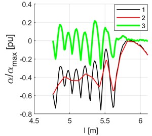
The first harmonic period equals the path along the switch, which is: 6.1068 – 4.7648 = 1.3420 m (Fig. 16). Wavelengths of successive harmonics are shorter by twice the value of the sampling period, 0.0123 m. The graphs provided are relative to the number of waves per one unit of length [1 m], being a parameter defined as follows: . The solid line in Fig. 18 marks a half of the root-mean-square value of the varying component. The functions shown in graphs can be assigned the following characteristics:
• Root-mean-square value of a fragment of the yaw angle curve which corresponds to running at a switch,
• Root-mean-square value of a varying component,
• Wavelength at which the cumulative distribution function of the root-mean-square value of harmonics reaches half of its value.
The above signal characteristics can be expressed in the following equation:
where: – wheel set yaw angle (Fig. 7(b)), – root-mean-square value of the signal fragment at a switch (graph 1, Fig. 16), – root-mean-square value of the varying component (graph 3, Fig. 16), – varying component amplitude (Fig. 17), – number of the varying component’s harmonics, – ordinal number of the harmonic on which the cumulative distribution function of the root-mean-square value reaches half of the cumulative value (Fig. 18), – number of waves of the FFT harmonic function for a path section of 1 m, – number of waves for the th harmonic, l – instantaneous value of path, – path covered.
Fig. 17FFT amplitude spectrum of the varying component of normalised yaw angle α/αmax(graph 3, Fig. 16)
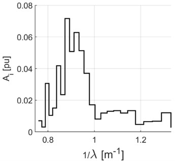
Fig. 18Cumulative distribution (function) of the root-mean-square value of the FFT distribution harmonics in the function of the number of waves Λ= 1/λ for the varying component of yaw angle in periods when the vehicle is running at switches, λ – wavelength [m]
![Cumulative distribution (function) of the root-mean-square value of the FFT distribution harmonics in the function of the number of waves Λ= 1/λ for the varying component of yaw angle in periods when the vehicle is running at switches, λ – wavelength [m]](https://static-01.extrica.com/articles/20577/20577-img30.jpg)
For the normalised signal fragment shown in Fig. 16, the values of the indicators in question are as follows: 0.2173 Pu, 0.1023 Pu; 0.8690 1/m.
The secondary effect caused by the vibrations is the increase in the power of lateral motion of tyres (Fig. 14). A characteristic feature of its behaviour may be the energy of this impact, expressed as follows:
where: – energy lost in the wheel tyre tread, – power of lateral forces (Fig. 14), – period of motion.
8. Results of the model parameter sensitivity analysis against the characteristics of torsional vibrations of wheel set axles
The aforementioned measures of characteristics (root-mean-square value and harmonic wavelength at which the rms value’s cumulative distribution function reaches half of the cumulative value) that have been applied with reference to the yaw angle signal for the period of time when the vehicle is running at a switch or for its transient component provide information on the force of torsional vibrations of the running wheels’ axle. On the other hand, the wheel tyre tread energy loss coefficient implies the tread wear. The above indicators transform the simulation results (on the pre-assumed structural parameters) into measures of characteristics of wheel axles’ torsional vibrations as well as of the wheel tyre tread wear. By that means, they also define the functions which depend on the parameters of simulation of the dynamics model (control variables of the parameter sensitivity analysis). The model parameter sensitivity analysis consists in studying the variability behaviour of these functions. The scope of the analysis may extend over all structural parameters, or it may be narrowed down to a limited group of parameters which exert the most significant impact on the force of vibration and wear of treads in running wheels.
Fig. 19, 20 provide graphs of functions of pre-defined quality indicators (4) and 1/ (5) depending on the coefficient of scaling of the tyre’s lateral grip and the coefficient of torsional elasticity and torsional damping of the wheel axle kingpin. Fig. 19 provides a graph of the values of coefficient (4) which describes the root-mean-square value of the varying component of the fragment of the yaw angle curve in periods when the vehicle is running at switches 1-3. What Fig. 19 implies is that function (4) assumes the lowest values for the values of control variables from the range of ≥ 1.0, ≥ 1.0 (while the local minimum is located in the vicinity of point 1.2, 2). Fig. 20 provides a graph of the function of wavelength 1/ (5) for half the root-mean-square value of the FFT cumulative distribution function of the varying component. With reference to Fig. 20, one can establish that the function assumes the lowest values under identical conditions as the function of indicator (4) shown in Fig. 19. It may be generally claimed that within the range of values of control variables, i.e. where ≥ 1.0, ≥ 1.0, the varying components of yaw angles in the periods when the vehicle is running at switches attain the best assessment indicators for vibration intensity.
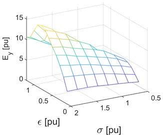
Fig. 21 provides a graph of the function of energy losses due to the lateral forces acting in wheel tyre treads (6). The coefficient assumes the lowest value on 0.1 (i.e. under conditions nearing to those of absence of lateral grip). However, this function also has a local minimum within the range of values of 0.8, 1.
Fig. 19Graph of function ΨZ (4) of the root-mean-square value of the varying component of the yaw angle curve for periods of running at switches
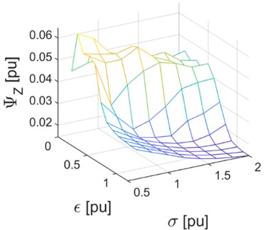
Fig. 20Graph of the function of wave number ΛN= 1/λN (5) for the varying component of yaw angle for periods of running at switches

9. Discussions
This article addresses results of an analysis of behaviour of variability of three qualitative indicators. Two of them, i.e. (4) and (5), are measures of the characteristics of intensity of the torsional vibrations observed in wheel sets, while the third one, i.e. (6), is a measure of energy loss for lateral forces acting in wheel tyre treads. What has been assumed to function as control variables is the lateral grip coefficient of tyres as well as the coefficient of torsional elasticity and torsional damping of the wheel axle kingpin. The analysis performed under the study, whose results have been discussed, is basically a multi-criteria analysis which additionally enables the set of decision making parameters to be extended. The article has demonstrated that in cases where the main goal underlying the choice of values of structural parameters is to limit the force and velocity of torsional vibrations of wheel set axles, then coefficients and should assume values from ranges ≥ 1.0, ≥ 1.0. In the said ranges of the coefficient values, one can also observe a trend of decreasing values of the indicators discussed (they are decreasing functions). This is not the case of the energy loss coefficient corresponding to the lateral forces acting in wheel tyre treads. Within the said range of values of control variables ( ≥ 1.0, ≥ 1.0), the energy loss coefficient value shows an increase trend. In order to accurately establish the optimum values of coefficients and (constituting a compromise between intensity of wheel set vibrations and the anticipated service wear of wheel tyre treads), one must first assume specific values of weight factors for individual coefficients.
Fig. 21Graph of function Ey (6) of the energy loss from wheel tyre treads
10. Conclusions
This publication provides a discussion on a narrow sphere of research concerning the analysis of running properties of PRT vehicles. These properties are inextricably linked with certain structural characteristics: non-profiled and independently revolving running wheels, wheel sets with turning axles, guiding along the guideway by means of a set of rollers featuring the passive switch system. They may trigger undesirable phenomena during travel, particularly torsional vibrations of wheel set axles, yawing or sticking. The paper discusses how it is theoretically possible to select appropriate structural parameters of a vehicle model in order to eliminate the negative effects of torsional vibrations. In order to fulfil this goal, several tasks must first be accomplished. One should develop a model of vehicle dynamics as well as a guideway edge model, perform simulation tests, determine the characteristics of torsional vibrations which can be revealed in the simulation results, demonstrate the relevant methods enabling these characteristics to be extracted, define coefficients creating a system of the aforementioned characteristics that is convenient to use, and finally, analyse sensitivity of the model parameters against pre-established assessment criteria. It has been demonstrated that the proposed procedure can be successfully used to determine ranges of optimum values of structural parameters (against the criterion of minimised effects of torsional vibrations).
The research will continue. And since a scaled physical model of a PRT system has been built at the Warsaw University of Technology, the model proposed will be validated following adequate measurements. It is assumed that the experience acquired in the fields of design and research while modelling scaled PRT vehicles can be utilised in practice when designing PRT infrastructure of real-life dimensions. What has recently been planned under the state government’s project known as “Elektro-Mobilność” is to implement a pilot PRT system dedicated to the municipality of Rzeszów.
References
-
2getthere Official Website – Floriade PRT, https://www.2getthere.eu/.
-
Lowson M. V. Engineering the ULTra system. Ingenia, Vol. 13, 2002, p. 6-12.
-
Gustafsson J. Vectus – intelligent transport. Proceedings of the IEEE, Vol. 97, Issue 11, 2009, p. 1856-1863.
-
Eriksson A. Identification of Environmental Impacts for the Vectus PRT System Using LCA. 2012, http://www.w-program.nu/filer/exjobb/Anders_Eriksson.pdf.
-
ModuTram Test Track. Atra Advanced Transit Association, 2014, http://www.advancedtransit.org/library/news/modutram-test-track/.
-
Anderson J. E. Transit Systems Theory. D.C. Heath and Company Lexington, Massachusetts, 1978.
-
Irving J. H., Bernstein H., Olson C. L., Buyan J. Fundamentals of Personal Rapid Transit. Lexington Books, D.C. Heath and Company Lexington, Massachusetts, 1978.
-
Burke C. G. Innovation and Public Policy – The Case of Personal Rapid Transit. D.C. Heath and Company Lexington, Massachusetts, 1979.
-
Choromański W. PRT Transport Systems. WKiŁ, Warszawa, 2015, (in Polish).
-
Cabinentaxi PRT System. Cabinentaxi Corporation, http://faculty.washington.edu/jbs/itrans/cabin.htm.
-
Elias S., Neuman E., Iskander W. Impact of People Movers on Travel: Morgantown – A Case Study. Transportation Research Record 882, 1982.
-
Lowson M. V. PRT for airport applications. TRB 84th Annual Meeting, Washington, 2005.
-
Richards B. Future Transport in Cities. First Ed., Taylor & Francis, 2001.
-
ATRA Advanced Transit Association, ATRA Advanced Transit Association Official Website – Systems, http://www.advancedtransit.org/advanced-transit/systems/.
-
Minderhoud M. M., Van Zuylen H. J. Preliminary assessment of the operation of a personal rapid transit system in Eindhoven. The IEEE 5th International Conference on Intelligent Transportation Systems, 2002, p. 428-433.
-
Li J., Chen Y. S., Li H., Anderson I., Van Zuylen H. Optimizing the fleet size of a personal rapid transit system: a case study in port of Rotterdam. 13th International IEEE Conference on Intelligent Transportation Systems, 2010, p. 301-305.
-
Furman B., Fabian L., Ellis S., Muller P., Swenson R. Automated Transit Networks (ATN): A Review of the State of the Industry and Prospects for the Future. MTI Report 12-31, 2014, http://transweb.sjsu.edu/project/1227.html.
-
Nikoniuk M. Synthesis of Contactless Energy Transfer System for the PRT Vehicle in the Traffic Conditions of the Automatic Transport Network. Ph.D. Thesis, Politechnika Warszawska, Wydział Transportu, 2018, (in Polish).
-
Anderson J. E. Control of personal rapid transit systems. Journal of Advanced Transportation, Vol. 32, Issue 1, 1998, p. 57-74.
-
Zhao K., Gang J., Wang Y., Lee D. Optimizing the link directions of personal rapid transit network. IEEE Transactions on Intelligent Transportation Systems, Vol. 19, Issue 10, 2018, p. 3414-3419.
-
Hollar S., Brain M., Nayak A. A., Stevens A., Patil N., Mittal H., Smith W. J. A new low cost, efficient, self-driving personal rapid transit system. IEEE Intelligent Vehicles Symposium (IV), 2017.
-
Hoang T., Nguyen T., Shiao Y. Simulation of intelligent merging control for personal rapid transit. 7th International Conference on Information Science and Technology (ICIST), Vietnam, 2017.
-
Schweizer J., Danesi A., Rupi F., Traversi E. Comparison of static vehicle flow assignment methods and microsimulations for a personal rapid transit network. Journal of Advanced Transportation, Vol. 46, Issue 2012, 2012, p. 340-350.
-
ECO-Mobilność – System PRT. Politechnika Warszawska Wydział Transportu, http://www.eco-mobilnosc.pw.edu.pl/pl_system-prt,24.html.
-
Choromański et al. Innovative and Environmentally Friendly Means of Transport. WKiŁ, Warszawa, 2015, (in Polish).
-
Kowara J. Simulation Research of Handling Characteristics and Dynamic Loads on Passengers in PRT Vehicles. Ph.D. Thesis, Politechnika Warszawska Wydział Transportu, Warszawa, 2015, (in Polish).
-
Kozłowski M., Choromański W., Kowara J. Analysis of dynamic properties of the PRT vehicle-track system, Bulletin of the polish academy of sciences. Technical Sciences, Vol. 63, Issue 3, 2015, p. 799-806.
-
Daszczuk W. B., Mieścicki J., Grabski W. Distributed algorithm for empty vehicles management in personal rapid transit (PRT) network. Journal of Advanced Transportation, Vol. 50, Issue 4, 2016, p. 608-629.
-
Kozłowski M. Simulation method for determining traction power of ATN-PRT vehicle. Transport, Vol. 33, Issue 2, 2018, p. 335-343.
-
Nikoniuk M., Kozłowski M. Energy properties of a contactless power supply in PRT (Personal rapid transit) laboratory model. Eksploatacja i Niezawodnosc – Maintenance and reliability, Vol. 20, Issue 1, 2018, p. 107-114.
-
Kamiński G., Przyborowski W., Staszewski P., Biernat A., Kupiec E. Design and test results of laboratory model of linear induction motor for automation personal urban transport PRT. Przegląd Elektrotechniczny, Vol. 93, Issue 3, 2017, p. 276-283.
-
Iwnicki S. Handbook of Railway Vehicle Dynamics. Taylor & Francis Group, London, 2006.
-
Tyremodels MF-TYRE & MF-SWIFT. TASS International, https://tass.plm.automation.siemens.com/ delft-tyre-mf-tyremf-swift.
Cited by
About this article

