Abstract
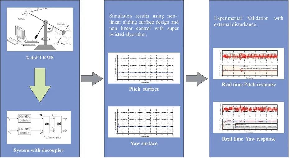
This paper proposes the design of a nonlinear sliding surface based on the principle of variable damping concept for 2-degree of freedom Twin Rotor Multiple input Multiple output System (2-dof TRMS). The implementation of the designed nonlinear sliding surface in real time is demonstrated. Super-twisting algorithm is applied in nonlinear sliding mode control. The nonlinear sliding surface enables the system trajectory to be highly robust and with the application of super-twisting algorithm in nonlinear sliding mode controller (SMC), the designed controller has minimized the problem of chattering considerably. The system is modeled in such a way that it includes all nonlinearities and coupling effects. A decoupler is designed to nullify the coupling effect. This scheme is capable of reducing both the settling time and peak overshoot simultaneously for 2-dof TRMS. The scheme also reduces the chattering. The proposed method is compared with the design using PID controller. The applicability of the designed nonlinear sliding surface and nonlinear SMC with super-twisting algorithm have been tested both in simulation and in real time. This research paper is mainly dealing with the modeling of Twin rotor MIMO system by including all nonlinearities and coupling effects, the decoupler design for 2-dof TRMS, the design of nonlinear sliding surface for 2-dof TRMS and application of super-twisting algorithm in nonlinear sliding mode control for 2-dof TRMS.
Highlights
- Modeling of highly nonlinear 2-dof TRMS system by incorporating all nonlinearities
- Increase in robustness with the application of nonlinear sliding surface based on variable damping ratio concept in 2-dof TRMS system
- Reduction in chattering in the pitch and yaw angle position tracking with the application of super-twisting algorithm in nonlinear sliding mode control
- Simultaneous reduction in both settling time and peak over shoot in the pitch and yaw angle position tracking with the use of nonlinear sliding surface based on variable damping ratio concept
1. Introduction
The 2-degree of freedom Twin Rotor MIMO System (2-dof TRMS) is a set up designed for carrying out control experiments in laboratories. The behavior of TRMS resembles to that of a helicopter whose performance is described as highly unstable nonlinear dynamics with heavy cross-coupling effects [1]. Hence controlling of TRMS System always poses a challenge.
PID Controller is one of the control algorithms mostly used in 2-dof TRMS [2-4]. The drawbacks of the PID controller design are the lack of specific methods to tune proportional, integral and derivative gains of PID controllers for 2-dof TRMS, the existence of high overshoot and the existence of high settling time. In literature [5, 6], the authors have proposed inventive methods to tune the proportional, integral and derivative gains of PID controllers. But there exists a small percentage of overshoot and high settling time. These drawbacks are claimed to have been eliminated by using sliding mode control (SMC) as presented in [7]. Although they could attain a good tracking performance with less overshoot, the scheme failed to reduce settling time because of the selection of linear switching surface for a nonlinear system. The above-mentioned high overshoot along with the reduced settling time is achieved in [8] using fuzzy sliding mode controller for 2-dof TRMS. Even if 2-dof TRMS with fuzzy sliding mode controller alleviates chattering effects and remain robust to external disturbances, it has the drawback of increased number of membership functions. In [9], the authors have developed T-S fuzzy model-based controller. The authors in [10] have proposed a method of evolving nuero-fuzzy network with fast learning adaptive procedure. In literature [11], the authors have designed robust H-Infinity algorithm. The state feedback linearization controller by defining optimal sliding surface have been designed in [12]. Although it shows good performance, it suffers from high settling time in real time application. As the accuracy in the improvement of the system performance depends on the methods upon which the surface is defined, the control engineers adopted alternative methods. In [13], the authors proposed an adaptive second order sliding mode controller where the coupling effect factor between pitch and yaw is taken as uncertainty. Similarly, in [14] also the coupling effect factor is taken as uncertainty. The authors in [15] claim that the control action could reduce the coupling effect. But when the 2-dof TRMS system is analyzed, it is to be ensured that coupling effect of the system is nullified. In literature [16], although the authors nullified the coupling effect, they could not attain improvement in transient performance of 2-dof TRMS.
In this paper, the system has been modeled by including all nonlinearities and coupling effects. To reduce the cross-coupling effects, a decoupler is designed such that one reference signal, affects only one physical output. Highly robust nonlinear sliding surface and nonlinear sliding mode control with super-twisting algorithm are designed for 2-dof TRMS. The designed nonlinear sliding surface based on the principle of variable damping concept [17] is applied in 2-dof TRMS. The damping ratio is varied from initial low value to high value. The initial low value of damping leads to quick response and high value of damping thereafter leads to less settling time [17]. Sliding mode control always produces chattering. Chattering in the control signal of 2-dof TRMS produce heat and mechanical vibration of the system which eventually results into mechanical damage in real time application. Therefore, the Sliding mode controller (SMC) is designed using nonlinear SMC with super-twisting control to reduce chattering. Linear portion of the nonlinear sliding surface is designed using the optimal sliding surface design procedure [18] and the super twisting controller available in [19] is introduced in the nonlinear SMC.
In Section 2, dynamics of 2-dof TRMS is explained. Modeling of 2-dof TRMS is presented in Section 3. Section 4 gives description of decoupler design. The nonlinear surface design procedure is dealt in Section 5. Section 6 explains the nonlinear sliding mode controller with the super-twisting algorithm applied to 2-dof TRMS. The simulation results of these decoupled 2-dof TRMS are presented in Section 7. In Section 8, the real time implementation results are presented. Finally concluding remarks are presented in Section 9.
2. Dynamics of 2-dof TRMS
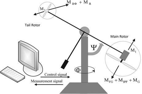
Fig. 1 shows the Twin Rotor MIMO (2-dof TRMS) system consisting of two rotors; one main rotor and the other tail rotor [16]. The support stiffness of the TRMS is ignored as the considered system is a rigid one. [20] The main rotor produces a lifting force allowing the beam to rise vertically while the tail rotor is used to make the beam to turn left and right around the horizontal axis. The dynamics of 2-dof TRMS in [1, 16] is once again provided below for quick reference.
The moment due to vertical movement of 2-dof TRMS consist of moment due to pitch angle acceleration, moment due to non-linear characteristic , moment due to gravity , moment due to frictional force and gyroscopic moment . The following equation shows the relation between these variables:
The moment due to nonlinear static characteristic is related with the torque developed in the main rotor as:
where and are constants. The relation between gravity moment and pitch angle is given by:
The relation between frictional force moment , pitch angle velocity and yaw angle velocity is given by:
The relation between gyroscopic moment and yaw angle velocity is given by:
Similarly, the moment due to horizontal movement is given as:
Fig. 1TRMS System
Here represents the yaw angle acceleration, represents the moment due to nonlinear static characteristic of tail rotor, represents frictional force moment and is cross-reaction moment. The moment due to nonlinear static characteristic of tail rotor is related with torque developed in the tail rotor as:
where and are constants. The relation between frictional force moment and yaw angle velocity is given by:
The following equation approximate the cross-reaction moment:
where and represent the cross-reaction moment parameters. The modeling of 2dof-TRMS is done by assuming the operating point as origin. The state space modeling of 2-dof TRMS is dealt in Section 3.
3. State space modeling of 2-dof TRMS
There are two types of modeling namely transfer function modeling and state space modeling. Since the system is MIMO and highly nonlinear the state space modeling is designed first and the transfer function model is calculated from the state space model. From the above set of Eqs. (1-9), it is evident that the system is nonlinear. The state model consists of state differential equation and output equation.
The state differential equation is given by:
The output equation is given by:
where represents the linear part of the system in state space representation and represents nonlinear part. The matrix represents the system matrix, accounts for the input distribution matrix, is the state vector, is the output vector and is the control input. is given by: , where is the input (control) voltage applied to main rotor and is the input (control) voltage applied to tail rotor. The maximum and minimum input (control) voltages for both main rotors and tail rotors are between –2.5 V and +2.5 V as per the specification in TRMS manual [1].
The state vector of 2-dof TRMS is given by:
where: : pitch angle of 2-dof TRMS; : yaw angle of 2-dof TRMS; : pitch angle velocity; : yaw angle velocity; : torque developed in the main rotor; : torque developed in the tail rotor.
The output vector is given by:
The derivative of the state vector is give is given by:
The values of , , , , , in terms of , , , , , can be calculated as follows.
The set of Eqs. (1-9) are rearranged and divided into linear and nonlinear part. The derivative of () is given by:
Eq. (1) is rearranged as follows:
Substituting all available values from Table 1, becomes:
The derivative of () is given by:
Eq. (6) can be rearranged as:
Substituting all available values from Table 1, becomes:
The time derivative of torque developed in main rotor is given by:
where , are the main rotor parameters. is the main rotor gain [1].
Substituting all available values from Table 1:
The time derivative of torque developed in tail rotor is given by:
where , , are the tail rotor parameters. is the tail rotor gain [1].
Substituting all available values from Table 1:
The values of matrices , , and can be calculated from Eqs. (15)-(24). The values of the above mentioned matrices are calculated as:
The nonlinear part of related with pitch angle acceleration is represented by . The nonlinear part of related with yaw angle acceleration is represented by :
Taking the above set of Eqs. (29)-(30) and substituting all the values for the parameters of 2-dof TRMS as per Table 1:
The transfer function of linear part of the above system is calculated using the equation in pole-zero form is given by:
Table 1TRMS parameters
Symbol | Parameter | Values |
Moment of inertia of vertical rotor | 6.8×10⁻² kg-m2 | |
Moment of inertia of horizontal rotor | 2×10⁻² kg-m2 | |
Static characteristic parameter | 0.0135 | |
Static characteristic parameter | 0.0924 | |
Static characteristic parameter | 0.02 | |
Static characteristic parameter | 0.09 | |
Gravity momentum | 0.32 N-m | |
Friction momentum parameter | 6×10⁻³ N-m/rad | |
Friction momentum parameter | 1×10⁻¹ N-m/rad | |
Friction momentum parameter | 1×10⁻² N-m/rad | |
Gyroscopic momentum parameter | 0.05 sec/rad | |
Motor 1 gain | 1.1 | |
Motor 2 gain | 0.8 | |
Motor 1 denominator parameter | 1.1 sec | |
Motor 1 denominator parameter | 1 | |
Motor 1 denominator parameter | 1 | |
Motor 1 denominator parameter | 1 | |
Cross- reaction momentum parameter | 2 | |
Cross-reaction momentum parameter | 3.5 | |
Cross-reaction momentum gain | –0.2 |
It can be seen that the system is modeled by including all nonlinearities and coupling effects. The design of decoupler is to be done for nullifying the coupling effect. Also, the transfer function of decoupled system is to be find out. These are discussed in Section 4.
4. Design of decoupler for 2-dof TRMS
In this Section, a decoupler for linear part of 2-dof TRMS is designed. From the Eq. (32), it is to be noted that the cross-coupling between pitch and yaw angles for the nonlinear part of 2-dof TRMS is negligible as compared with the linear part of 2-dof TRMS. Hence in this work the cross-coupling effect for the nonlinear part of 2-dof TRMS is avoided while calculating the parameters of the decoupler.
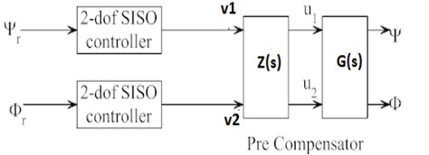
The transfer function for linear part of 2-dof TRMS in Eq. (32) reveals that there exists coupling between the yaw and input signal () given to pitch. The above coupling effects can be nullified by suitably designing a decoupler known as pre-compensator which is dealt in this Section. For a given MIMO plant , a method to design pre-compensator (decoupler) is available in [16]. Fig. 2 represents the system with decoupler. The and , represent the reference pitch and yaw angle respectively and these are given as controller inputs to two 2-dof SISO controllers. The controller outputs, and are the inputs to the pre-compensator (decoupler). The decoupler outputs are and respectively, and these are given as the inputs to the system. While designing the decoupler , it is to be ensured that the unstable poles and zeroes are not cancelled against each other. To avoid the cancellation of unstable poles and zeroes the ‘minimal-di’ (minimum number of unstable poles and zeroes including those at infinity) is calculated first and then decoupler is designed. The method of calculation of decoupler [16] is applied here. The decoupler for 2-dof TRMS is given by:
where and is the system transfer function. From the Eq. (32), it is obvious that has unstable poles at 0. The stable poles are at –0.0881 and –0.9090. The pole at –0.0881 which is very near to zero is also considered for the calculation of ‘’. The zeroes are at infinity. The terms necessary for the design of ‘’ for this model are calculated as per [16] as:
Fig. 22-dof TRMS with decoupler
These terms are used for calculating the factors that must be present in ‘’:
Here represents the number of poles present in of . From the design procedure consists of three poles. Similarly represents the number of poles present in of . also consists of 3 poles.
The factors that must be present in ‘are calculated as:
This equation represents that there is a pole at origin in the term of :
This equation represents that there is a pole at the origin in the term of :
This equation represents that there is a pole at 0.08819 in the term of minimal :
This equation represents that there is no pole at 0.08819 present in the of minimal .
From the above design procedure for ‘’ it is noted that and consist of three poles and three zeros. The poles that are present in are one at origin as 1, and other one at –0.08819 as 1. The third one is assumed at and the zeros of are at infinity. The value of is assumed to be as 0.9090. The reason why 0.9090 considered is that the value of –0.9090 is present in pitch angle transfer function as well as in the coupling term of TRMS system. Now of the ‘’ becomes:
Similarly consists of three poles with one at origin and three zeroes are at infinity. For simplicity it is assumed that 0.9090 and 0.9090. The reason why 0.9090 and 5 considered is that the value of –0.9090 and –5 are present in yaw angle transfer function as well as in the coupling term of TRMS system. Now of the ‘’ becomes:
Now the ‘’ is given by :
The pre-compensator (decoupler) is calculated from Eq. (33) as:
With the introduction of decoupler the coupling term of 2-dof TRMS system is made to be zero. Now the net transfer function of the 2-dof TRMS system is obtained as:
To match with the system designed , the first row is multiplied with 1.358 and the second row with 3.6. Then the modified transfer function of the decoupled system becomes:
The Eq. (47) shows the transfer function of the decoupled system. It can be seen that the terms corresponding to the coupling effect between pitch and yaw of 2-dof TRMS are nullified. After obtaining the transfer function model of the decoupled system the next step is the design of the nonlinear sliding surface which is dealt in Section 5.
5. Design of nonlinear sliding surface for 2-dof TRMS
The performance improvement in 2-dof TRMS is obtained with nonlinear sliding surface design based on variable damping ratio concept [17]. This system involves the design of nonlinear sliding surfaces for both pitch and yaw angles. Since the designed sliding surface is asymptotically stable in the sense of Lyapunov, the unmodeled dynamics like localized defects (LOD) [21] can be assumed to be of no effect in the performance of TRMS. The design of nonlinear sliding surfaces in both mentioned cases are synthesized adopting the approach mentioned in [17].
Step 1. Design of Pitch angle nonlinear sliding surface.
From the decoupled transfer function model Eq. (47), the main rotor transfer function for linear part of TRMS is given by:
For writing the state model of pitch the non-linearity is added with the linear part of the pitch. The state model of the pitch is given by:
Output equation for pitch is given by:
The switching function for pitch is given by:
where and is the nonlinear sliding surface matrix. The system represented by the Eq. (48) is a third order system. Generally regular form approach is employed to bring down the higher order for simplicity. For the system considered, different sets of state variables are employed using to apply regular form approach. The is related to the conventional pitch angle state vector as:
here is the orthogonal matrix used for coordinate transformation. Now the regular form of the Eq. (49) becomes:
where:
And , . The associated sliding surface in regular form can be expressed as:
where:
The term in Eq. (56) corresponds to nonlinear part of the surface and to linear part of the surface. The sliding surface matrix is written as:
The pitch surface for the 2-dof TRMS can be represented as:
where is a positive definite function. The represents the nonlinearity function associated with the nonlinear part of sliding surface. The selection of is done in subsection 5.1. The value of linear part of sliding surface is calculated using the quadratic minimization technique which is explained in [18] is given below.
During sliding mode the sliding surface 0, then Eq. (55) becomes:
Then Eq. (60) can be written as:
The value of is calculated by minimizing the performance measure using the system constraint equation which is detailed below:
where represents the time at which the sliding mode commences. The matrix is the performance index matrix. It is selected to minimize the deviation of the final value of system from the desired value. The value of is assumed as identity matrix as:
The performance index matrix is transformed and partitioned in compatibility with as:
where:
Now the performance measure represented in coordinate transform is given by:
The modified performance measure can be written as:
where:
Now the performance measure is to be minimized according to the constrained equation which is given below:
The modified constraint equation becomes:
where:
Substituting all available values in Eq. (72):
A unique positive definite solution ‘’ is guaranteed for the algebraic matrix Ricatti Eq. (74) as:
Substituting all above values in Ricatti Eq. (74) a unique positive definite solution can be obtained as:
The expression for partition is given by:
Comparing the Eqs. (61) and (76):
Inserting the value of in Eq. (77), can be calculated as:
The Eq. (78) shows the linear part of the surface.
In Eq. (56), is a positive definite matrix satisfying the Lyapunov equation which is given below:
where is a positive definite matrix and is selected as in [18]:
By substituting all the values of , , , and in the Eq. (74), is calculated as:
The next sub Section deals with the nonlinearity function associated with the nonlinear sliding surface given in Eq. (59).
5.1. Nonlinearity function
The nonlinearity function is used to change the system closed loop damping ratio from its initial low value to high value as the output varies from its initial and approaches final value [17]. This Section presents nonlinearity function for pitch and yaw. represents the pitch angle nonlinearity function and represents the yaw angle nonlinearity function. It should satisfy the following properties as per [17].
It should vary from 0 to as the output approaches the set point (final value) from its initial value where . It should be differentiable with respect to which ensure the existence of sliding mode. The possible choice of as:
where and are positive constants. should have a large value to ensure a small initial value . Similarly, the nonlinearity function for yaw is given by:
Substituting all the available values in Eq. (59), the nonlinear sliding surface for pitch is obtained as:
Step 2: Design of yaw angle nonlinear sliding surface.
The procedure for the design of nonlinear sliding surface for yaw is carried out in the same way as that for the nonlinear sliding surface design of pitch. The nonlinear sliding surface of yaw is obtained as:
5.2. Stability analysis of nonlinear sliding surface
The stability of the designed nonlinear sliding surface is to be ensured before designing the nonlinear sliding mode controller. And the same is done using the Lyapunov stability analysis.
Proof: let the positive definite Lyapunov function be:
where is positive definite and it is chosen based on condition satisfying the Lyapunov Eq. (79). The derivative of Lyapunaov function becomes:
Substituting for in Eq. (87), becomes:
Substituting in Eq (88), – becomes:
As is negative definite by definition and , the second term of Eq. (84) becomes negative definite matrix. Adding this term with negative definite matrix , results in negative definite matrix. Therefore, it can be written as . Thus, the designed pitch angle nonlinear sliding surface for 2-dof TRMS is stable in the sense of Lyapunov. The stability of yaw angle nonlinear sliding surface can be proved by the same procedure. Thus, it is proved that the designed nonlinear sliding surface for 2-dof TRMS is stable and satisfies the Lyapunov stability analysis.
In this Section the nonlinear sliding surface is designed based on variable damping concept. The linear part of the surface is designed using the quadratic minimization procedure. The nonlinearity function is selected as per [17]. The stability of nonlinear sliding surface designed is tested using Lyapunov stability analysis. In addition to the design of nonlinear sliding surface, the design of nonlinear sliding mode controller is also to be done which is explained in Section 6.
6. Design of nonlinear sliding mode controller with super-twisting algorithm for 2-dof TRMS
The main problem of sliding mode control is chattering in control signal. High chattering affects the mechanical part of the system in real time. To reduce such chattering, the higher order sliding modes are introduced. The main disadvantage of using higher order sliding mode is the difficulty in gathering information of derivatives in real time. But the super-twisting algorithm does not require the information regarding the derivatives. This super-twisting control is a continuous control ensuring all properties of first order sliding mode control.
The nonlinear SMC for 2-dof TRMS is designed adopting the control structure envisaged in [18] but with a modification. Instead of the signum function used in [17] super-twisting algorithm is adopted in this work to reduce chattering [19]. In the existing nonlinear SMC mentioned in literature [17], a super-twisting controller [19] is incorporated which is explained below:
The above equation forms the nonlinear sliding mode controller with super-twisting algorithm introduced, where represents the super-twisting control to reduce chattering.
The following values are chosen for , as 6, 4 and 0.9. The value of is chosen by considering condition where is maximum bound of uncertainty for pitch [17]. The maximum bound of uncertainty for pitch is calculated to be 0.875. The value of and are chosen by trial and error method. Substituting all available values in Eq. (90), becomes:
Similarly yaw control is given by:
where 6 and 4 are the values obtained by trial and error method. The value of 1.7. The value of is chosen by considering condition where is maximum bound of uncertainty for yaw [17]. The maximum bound of uncertainty for yaw is found to be 1.68. Substituting all available values in Eq. (92), becomes:
The next Section deals with the simulation results by the application of nonlinear sliding surface for 2-dof TRMS and design of nonlinear sliding mode controller with the introduction of super-twisting controller.
7. Simulation results and discussion
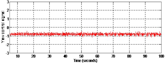
The simulation has been done for 100 seconds by taking unit step as reference input and the results are plotted for 2-dof TRMS. Fig. 3 shows the pitch control input when a matched disturbance of is added at 50 seconds. It is evident from the figure that the magnitude of pitch control signal is in between 1 V and 2.5 V which is within the prescribed control limit 2.5 V and –2.5 V [1]. Similarly, Fig. 4 shows the yaw control input when a matched disturbance of is added at 50 seconds. It is clear from the figure that the magnitude of yaw control signal is in between –0.5 V and –1 V. Since the control inputs generated for both pitch and yaw are within the control limit prescribed by the manufacturer of 2-dof TRMS [1], the implementation can be done in real time.
Fig. 3Pitch control (non-linear sliding surface design)
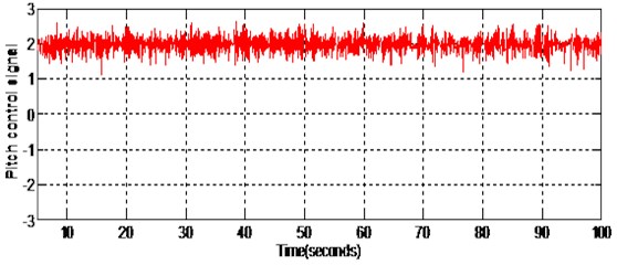
Fig. 4Yaw control (non-linear sliding surface design)
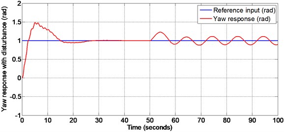
Figs. 5-6 show the pitch angle and yaw angle tracking responses respectively when the disturbance is given at 50 seconds. The pitch response settles in 8 seconds and yaw response settles in 7 seconds. It is noted that there is no initial overshoot and undershoot in both pitch and yaw responses. The disturbance of is given to both pitch and yaw through input channel (matched disturbance) at 50 seconds. Even when the disturbance is applied, both the outputs track the corresponding reference inputs. This verifies the in-variance property of the designed sliding surface.
Fig. 7 shows the pitch angle nonlinear sliding surface. During sliding mode the state vectors for pitch angle will slide along the designed sliding surface and keeps the tracking error to a minimum value. Fig. 8 shows the pitch angle nonlinear sliding surface with initial portion of the figure enlarged.
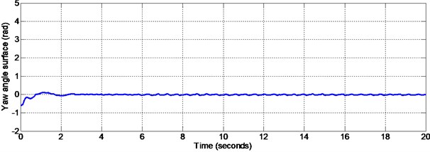
Fig. 9 shows the yaw angle nonlinear sliding surface. During sliding mode the states of yaw angles will slide along the designed sliding surface and keeps the tracking error to a minimum value. Fig. 10 shows the yaw angle nonlinear sliding surface with the initial portion of the figure enlarged. Also, the pitch and yaw angle responses will not be affected by the disturbances given to the system since the state trajectory slides along this nonlinear sliding surface designed.
Fig. 5Pitch response with matched disturbance given at 50 seconds (non-linear sliding surface design)
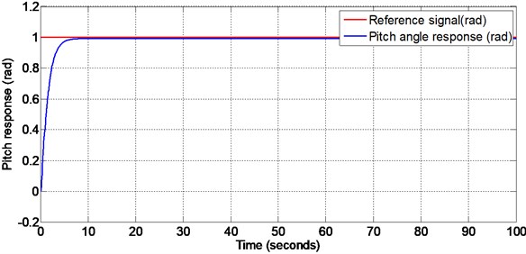
Fig. 6Yaw response with matched disturbance given at 50 seconds (non-linear sliding surface design)
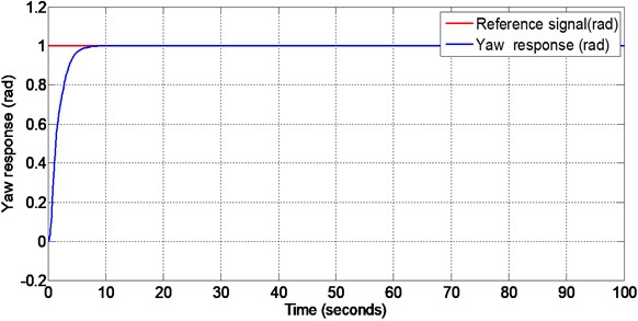
Fig. 7Pitch surface with matched disturbance given at 50 seconds (non-linear sliding surface design)
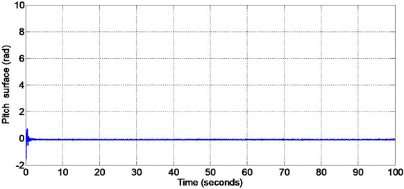
Fig. 8Initial portion of pitch surface (non-linear sliding surface design)
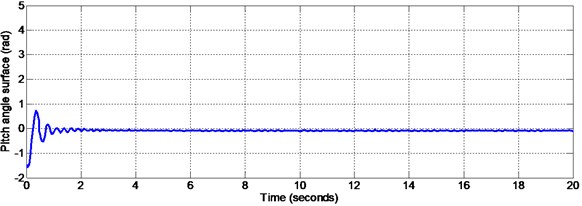
Fig. 9Yaw surface with matched disturbance given at 50 seconds (non-linear sliding surface design)
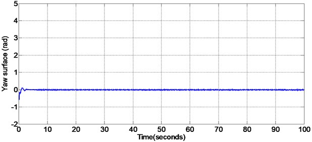
Fig. 10Initial portion of the yaw angle surface (non-linear sliding surface design)
PID controller is designed using appropriate tuning method. The values of proportional constant , integral constant and derivative constant are tuned as 2.5, 4, 7 for pitch PID controller design and 2.2, , for yaw PID controller design. A disturbance of has been given at 50 seconds to both pitch and yaw through input channels and the responses are plotted. Figs. 11-12 are the responses of the pitch and yaw angles respectively when the disturbance is given at 50 seconds. From these responses it is observed that the initial overshoot and settling time are very high for both pitch and yaw. The settling time for pitch and yaw is found to be 28 seconds 40 seconds respectively. Both the pitch and yaw responses deviates from the reference signals after the application of matched disturbance at 50 seconds. Also, it is noted that high chattering occurs with the application of PID controller.
Fig. 11Pitch response with matched disturbance given at 50 seconds (PID controller design)
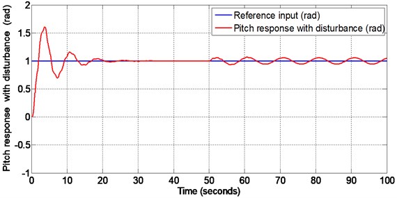
Fig. 12Yaw response with matched disturbance given at 50 seconds (PID controller with design)
8. Real time implementation
The real time implementation is done for 2-dof TRMS with the designed nonlinear sliding surface (as explained in section 5 of this paper) and nonlinear sliding mode controller with super-twisting algorithm (as explained in section 6) by using Advantech PCI1711 interfacing card. This card reads the 16 bit data from encoders. There are two blocks namely encoder (Analogue to digital) and decoder (digital to analogue) blocks. The encoder block has two outputs which are position of rotor in radians in the vertical and horizontal planes [1]. The control signals for pitch and yaw are given to the digital to analogue block. These encoder and decoder serves as an interface between the PC and external environment. The sensors senses the real time pitch and yaw angle positions. These real time angle positions sensed by the sensors are given to the encoders. The encoder delivers the discrete values corresponding to the interrupt service routine (ISR). The control algorithm operates according to the pulses distributed by the clock and the clock delivers the interrupt service routine.
Fig. 13Real time pitch response with external disturbance given at 32 seconds (non-linear sliding surface design)
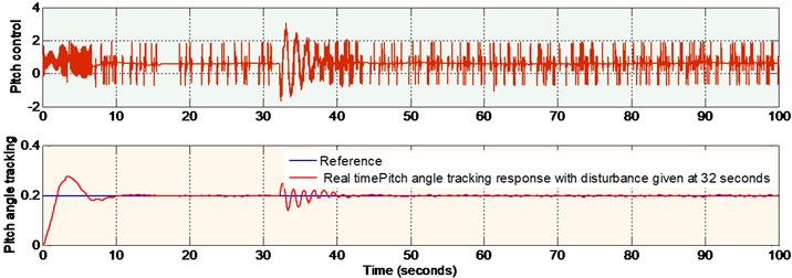
Fig. 14Real time yaw response with external disturbance given at 32 seconds
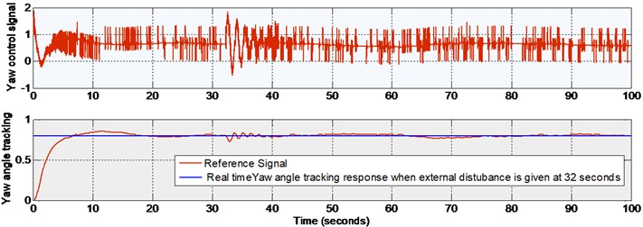
Since the system constraints are too high the operating region for pitch and yaw are to be fixed prior to the real time implementation. The operating region in radian for pitch is [–0.51 1.2] and for yaw is [–1.2 1.2] [14]. In this work lower values of reference inputs are applied. lower values, (0.2 radian for pitch and 0.8 radian for yaw) are applied in order to ensure safe operation of the TRMS.
The real time outputs (pitch and yaw angle positions) are taken from the encoder of PCI1711 card and are compared with the reference signals (both pitch and yaw). The error signals thus obtained are given to the nonlinear sliding surface with nonlinear sliding mode controller. The outputs of the controllers are given to DAC of PCI1711 card. Figs. 13-14, show the real time pitch angle and yaw angle tracking responses respectively and corresponding control signals, when the external disturbance (a manual force corresponding to 100 g) is given at 32 seconds. There is a small percentage of overshoot for the Pitch angle response at the beginning and this is due to the large moment of inertia of main rotor drum of 2-dof TRMS. The initial overshoot will be disappeared, and it will be settled within 10 seconds to the desired value. There is no overshoot for yaw angle response, and it settles in 20 seconds. The control signal is in between 2 V and –2 V for both pitch and yaw. It is noticed from the figures that both the outputs track the corresponding reference inputs. The deviation from the reference signals at the time of occurrence of the disturbance settles in 10 seconds. This verifies the in-variance property of the designed nonlinear sliding surface as explained in Section 5 of this paper. It is also observed that the chattering is reduced in the step responses of pitch and yaw angle responses due to the application of super-twisting algorithm in nonlinear SMC. The end results of this research work are explained in tabular form for ready reference as shown below.
Table 2Performance comparison
Pitch and yaw motion characteristics of 2-dof TRMS | Nonlinear sliding surface design with nonlinear SMC | Real time implementation of nonlinear surface with nonlinear SMC | PID controller design |
Settling time of pitch | 8 seconds | 10 seconds | 28 seconds |
Settling time of yaw | 7 seconds | 20 seconds | 40 seconds |
Overshoot of pitch | Nil | 40 percent | 50 percent |
Overshoot of yaw | Nil | Nil | 50 percent |
Robustness of pitch surface | The matched disturbance of does not affect the system. System become robust | System retains its steady value in 10 seconds even with the application of external disturbance. The system becomes robust. | The matched disturbance of affects the system. The System is not robust with the application of PID Controller. |
Robustness of yaw surface | The matched disturbance of does not affect the system. System become robust | System retains its steady value in 10 seconds even with the application of external disturbance. The system becomes robust | The matched disturbance of affects the system. The system is not robust with the application of PID controller |
Chattering in pitch response | Considerable reduction in magnitude | Considerable reduction in magnitude | |
Chattering in yaw response | Considerable reduction in magnitude | Considerable reduction in magnitude |
9. Conclusions
In this paper the modeling of the highly nonlinear 2 degree of freedom Twin rotor MIMO system (2-dof TRMS) by incorporating all the nonlinearities of the system is done. Also design of a decoupler which nullifies the coupling effect between pitch and yaw is done. In addition to that the design of a nonlinear sliding mode controller (SMC) with super-twisting algorithm using variable damping ratio based nonlinear sliding surface is done. The transient performance is improved, and chattering is reduced with the use of the proposed controller and it is verified both in simulation and in real time. It can be seen that the robustness of the system is improved and chattering in output response is reduced considerably. The nonlinear sliding surface proved to be stable satisfying the Lyapunov stability analysis. The proposed method for 2-dof TRMS has been tested in real time with the use of MATLAB toolbox and PCI1711 card. It is found that both the settling time and peak overshoot are reduced simultaneously with the use of nonlinear sliding surface and nonlinear SMC with super-twisting control.
In nutshell the system is modeled by including all nonlinearities and the effect of coupling between pitch and yaw of TRMS is nullified with the use of a decoupler. Also, the simultaneous reduction both in settling and peak overshoot is achieved by the use of nonlinear sliding surface based on variable damping ratio concept. The considerable reduction in chattering with the introduction of super-twisting algorithm in the nonlinear SMC is also achieved.
References
-
Twin Rotor MIMO System control Experiments: 33-949S. User Manual, Feedback Instruments Ltd., East Sussex, U.K., 2006.
-
Kuo B. C. Automatic Control Systems. 6th ed., Englewood Cliffs, Prentice-Hall, 1995.
-
Krohling R. A., Jaschek H., Rey J. P. Designing PI/PID controllers for a motion control system based on genetic algorithms. 12th IEEE International Symposium on Intelligent Control, Istanbul, Turkey, 1997, p. 125-130.
-
Huang M. T., Juang J. G. Application of GA and PID control to non-linear TRMS. Conference on Technologies and Applications of Artificial Intelligence, Taichung, Taiwan, 2002, p. 734-739.
-
Juang J. G., Huang M. T., Liu W. K. PID Control using presearched genetic algorithms. IEEE Transactions on Systems, Man, and Cybernetics: Systems. Vol. 38, Issue 5, 2008, p. 716-727.
-
Pramit Biswas, Roshini Maiti, Ariban Kolay, Koushik Das Sharma, Gautham Sarksr PSO based PID controller for TRMS. Proceedings of The International Conference on Control, Instrumentation, Energy and Communication, 2014, p. 56-60.
-
Su J. P., Liang C. Y., Chen H. M. Robust control of a class of nonlinear system and its application to a TRMS. Proceedings of IEEE International Conference on Industrial Technology, Bangkok, Thailand, 2002, p. 1272-1277.
-
Tao Chin-Wang, Taur Jin-Shiuh, Chang Yeong-Hwa, Chang Chia-Wen A novel fuzzy-sliding and fuzzy-integral-sliding controller for the twin rotor multi-input multi-output system. IEEE Transactions on Fuzzy Systems, Vol. 18, Issue 5, 2010, p. 893-905.
-
Deepak Kumar Saroj, Indrani Kar T-S fuzzy model based controller and observer design for a twin rotor MIMO system. IEEE International Conference on Fuzzy System, 2013.
-
Silva Alison, Caminhas Walmir, Lemos Andre, Gominde Fernado Real time nonlinear modeling of a twin rotor MIMO system using evolving Nuero-fuzzy network. IEEE Symposium on Computational Intelligence in Control and Automation, 2014.
-
John Lidiya, Mija S. Robust H-infinity control algorithm for twin rotor MIMO system. IEEE International Conference on Advance Communication Control and Computing Technology, 2014, p. 168-173.
-
Lisy E. R., Nandakumar M., Anasraj R. Design of an optimal sliding surface for Twin rotor MIMO system. 10th Asian Control Conference, Kota Kinabalu, Malasia, 2015.
-
Mondal S., Mahanta C. Adaptive second-order sliding mode controller for a twin rotor multi-input-multi-output system. IET Control Theory and Applications, Vol. 6, Issue 14, 2012, p. 2157-2167.
-
Samir Zeghlache, Abdderrahman Bougera, Muhammed Ladjal Sliding mode controller using nonlinear sliding surface applied to 2-dof Helicopter. Proceedings of 2nd International Conference on Electrical and Information Technologies, 2016.
-
Farah Faris, Abdelkrim Moussaoui, Boukhetala Djamel, Thadin Mohammed Design and real-time implementation of a decentralised sliding mode for Twin rotor multi input multi output, system. Journal of Systems and control Engineering, Vol. 231, Issue 1, 2017, p. 3-13.
-
Jatin Kumar Pradhan, Arun Ghosh Design and implementation of decoupled compensation for a twin rotor multiple -input and multiple-output system. IET Control Theory and Applications, Vol. 7, Issue 2, 2013, p. 282-289.
-
Fulwani D., Bandyopadhyay B., Fridman L. Non-linear sliding surface: toward high performance robust control. IET Control Theory and Applications, Vol. 6, Issue 2, 2012, p. 235-242.
-
Christopher Edward, Spergeon Sarah K. Sliding Mode Control Theory, Applications. Taylor Francis Ltd., London, 1998.
-
Kamal Shyam, Chalanga Asif, Moreno J. A., Fridman L., Bandopadhyay B. Higher order super-twisting algorithm. 13th International Workshop on Variable Structure Systems, 2014.
-
Mutra Rajasekhara Reddy, Srinivas J. Vibration analysis of support excited rotor system with hydro dynamic journal bearings. 12th International Conference on Vibration Problems, 2015.
-
Jing Liu, Yimin Shao Dynamic modeling for rigid rotor bearing systems with localised defect considering additional deformation at sharp edges. Journal of Sound and Vibration, Vol. 398, 2017, p. 84-102.
About this article

