Abstract
The submitted paper is devoted to the numerical modeling of the dynamic effects of moving vehicles on concrete pavements. The finite element method, namely the ADINA program, is used to model the problem. To solve the task, it is necessary to create a vehicle and a road computational models. The vehicle model is spacious and corresponds to a heavy truck of the Tatra type. The so-called single-layer road model on an elastic Winkler foundation is used. Concrete pavements are modeled using shell or solid elements. The output of the solution is the time course of the dynamic deflections at the individual points of the slab and internal forces and the stress states in the concrete slab at the individual time points of the solution. The calculation results for each computational model are compared to each other.
1. Introduction
Roads are typical transport structures subjected to the dynamic effect of moving vehicles. The most widespread types of roads are asphalt and concrete pavements. The moving load effect on pavements can be analyzed by numerical or experiment way. The determination of the dynamic response of road pavements to moving vehicle loads is a subject of current interest and importance, which are deals in many departments around the world [1-3]. To solve the task by the numerical way, it is necessary to create a vehicle and a road computational models. The models can be created in the sense of classical dynamic or in the sense of finite element method. The finite element method, namely the ADINA program [4], is used to model the problem in this paper. The vehicle model is spacious and corresponds to a heavy truck of the Tatra type. The road model can be created at different qualitative levels. The so-called single-layer road model on an elastic Winkler foundation is used. Concrete pavements can be modeled using shell or solid elements. Shell elements are more preferred in the case if the internal forces are needed to design the structure. The solid elements are more advantageous if the output is to be a more detailed analysis of the stress states of the structure. The base eight nodal elements may be used, or more nodal elements can be used depending on what output is expected from the solution. The output of the solution is the time course of the dynamic deflections at the individual points of the slab and internal forces and the stress states in the concrete slab at the individual time points of the solution. The calculation results for each computational model are compared to each other.
2. Vehicle computational model
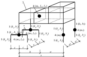
One of the most important steps for proper numerical simulation is to choose the appropriate model of the vehicle. The model should preferably represent the real vehicle. For the purposes of this simulation, the spatial model of the whole vehicle was chosen, Fig. 1. This numerical model of the vehicle has finite degrees of freedom and it is a combination of masses, springs, damping and 3D solid element. The numerical parameters used in this numerical model are as follows:
Geometry: 3.135 m; 1.075 m; 0.660 m; 0.993 m; 0.973 m.
Diagonal stiffness matrix: [143716.5; 143716.5; 761256; 761256; 1275300; 1275300; 2511360; 2511360; 2511360; 2511360]D [N/m] .
Diagonal mass matrix: [22950.0; 62298.0; 22950.0; 455; 455; 1070; 466; 1070; 466]D [kg, kg·m2].
Diagonal damping matrix: [9614; 9614; 130098.5; 130098.5; 1373; 1373; 2747; 2747; 2747; 2747]D [kg/s].
Fig. 1Vehicle computational model
a)
b)
3. Road computational model
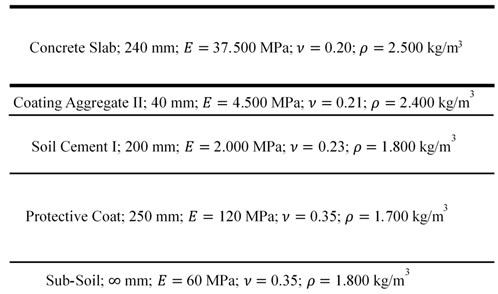
The subject of the modeling, in this case, is a concrete pavement consisting of nine slabs with planar dimensions of 6.8×4.9 m and a thickness of 0.24 m located in three rows next to each other. The total dimension of this area is 20.4×14.7 m. The solved area is covered by a finite element network measuring 0.425×0.490 m. The network represents 30 rows of elements parallel to the -axis and 48 rows of elements parallel to the -axis. The pavement composition in cross-section is shown in Fig. 2.
Fig. 2Pavement composition in cross-section
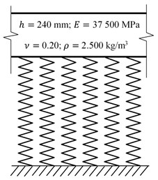
FEM computational models of concrete pavements can be created as a single layer or multilayer models. Single layer models are sufficient in case we want to analyze stress and strain states only in the reinforced concrete slab itself and we are not interested in stress and strain states in the individual subgrade layers. In this paper the single layer models of concrete pavement on elastic Winkler foundation are adopted, Fig. 3.
The modulus of compressibility [MN/m3] was calculated using the LAYMED program as follows [5]:
The layered half-space was loaded through an elastic steel circular plate, radius 40 cm, with the pressure 0.10 MPa. The value of the surface deflection of the considered layered half-space calculated by LAYMED is 0.471228 mm. Because the computed value of the deflection corresponds to the load transmitted by the elastic plate, the deflection must be recalculated to the rigid plate by a correction coefficient of 1.274. The elastic foundation is replaced by equivalent springs located in nodes of the FEM network. The area corresponding to one node is 0.425∙0.49 = 0.20828 m2. The stiffness of the spring located in the node is MN/m = 56.300.000 N/m. The mass intensity of the plate [kg/m2] is calculated as 2500·0.24 = 600.0 kg/m2. The damping is introduced into the calculation by the angular damping frequency in the value 0.1 rad/s.
Fig. 3Sigle layer computational model
The concrete slab can be modeled by a shell or solid elements. The Shell element is more advantageous in case if the outputs are to be the internal forces needed to dimensioning the slab (bending moments, shear forces, torsional moments). The solid element is more advantageous in case if the outputs are to be stress and strain states in the slab.
4. Results of the computation
The properties of the concrete slab are as follows: slab thickness 240 mm, modulus of elasticity of concrete 37 500 MPa, Poisson’s ratio 0.20, bulk density 2500 kg/m3. Other pavement layers are introduced into the calculation as an elastic Winkler foundation with compressibility modulus 270.3574 MN/m3. The stiffness of the spring located in the node is 56.300.000 N/m. The damping is introduced into the calculation as Rayleigh’s damping with 0.1 and 0.002.
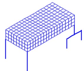
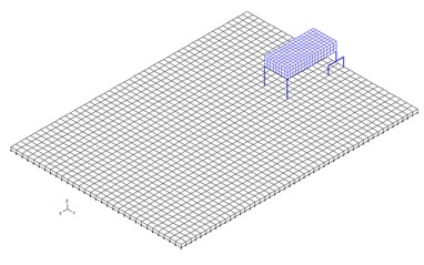
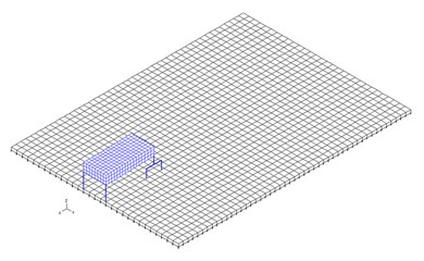
Fig. 4Vehicle in starting and ending position
a)
b)
The vehicle moves along the slab central axis with constant speed 65 km/h. The vehicle in starting and ending positions is shown in Fig. 4. Vehicle passage time along the slab is 0.86 s. The computation of the slab and vehicle response at riding of the vehicle along the slab was calculated in the environment of FEM System ADINA [4].
4.1. Model with shell elements
The used shell element has six DOFs in each node (three translational displacements in the , and directions, and three rotational deformations with respect to the , and axes). The output of the calculation is vertical displacements and internal forces. The time course of the vertical displacements in the middle of the slab at the speed of vehicle motion 65 km/h is shown in Fig. 5. Maximal displacement occurs at time 1.541 s in the value 0.063775 mm. Calculation time is 15 minutes.
Fig. 5Time course of the vertical displacements in the middle of the slab, shell elements
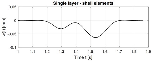
Fig. 6Vertical displacement in time t= 1.541 s, shell elements
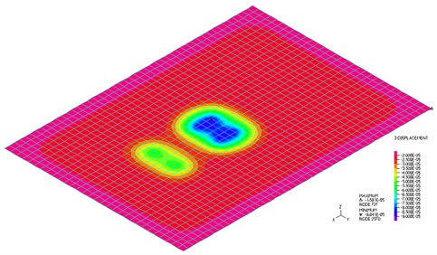
Fig. 7Bending moments myy parallel to the X-axis at time t= 1,541 s, shell elements
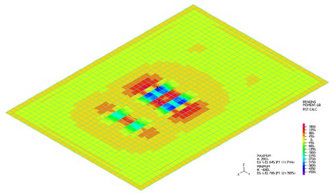
The isostructural surface of vertical displacements at the time 1.541 s when the maximal deflection in the middle of the slab occurs is shown in Fig. 6. The isostructural surface of bending moment parallel to the -axis at time 1.541 s when a maximal deflection in the middle of the slab occurs is shown in Fig. 7.
4.2. Model with solid elements
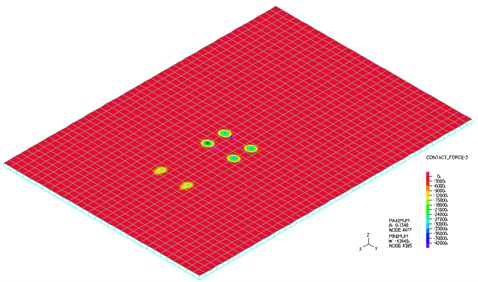
The used solid element has eight nodes with three DOFs in each node, total 24 DOFs. The output of the calculation is vertical displacements, stresses and contact force. The time course of the vertical displacements in the middle of the slab at the speed of vehicle motion 65 km/h is shown in Fig. 8. Maximal displacement occurs at time 1.544 s in the value 0.059536 mm. Calculation time is 7 minutes. The isostructural surface of vertical displacements at the time 1.544 s when the maximal deflection in the middle of the slab occurs is shown in Fig. 9. The isostructural surface of normal stresses at time 1.544 s when a maximal deflection in the middle of the slab occurs is shown in Fig. 10. The corresponding contact forces are shown in Fig. 11.
Fig. 8Time course of the vertical displacements in the middle of the slab, solid elements
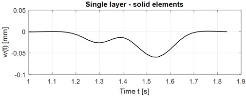
Fig. 9Vertical displacement in time t= 1.544 s, solid elements
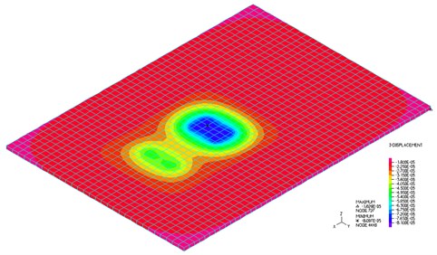
Fig. 10Normal stresses σzz at the time t= 1.544 s, solid elements
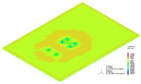
Fig. 11Contact force at the time t= 1.544 s, solid elements
4.3. Comparison of shell and solid element models
The results for FEM computational models using the shell and solid elements were mutually compared. The subject of comparison is the time course of vertical deflections in the middle of the slab. Comparison in graphical form is shown in Fig. 12. Comparison in numerical form is in Table 1. The solid model is a bit stiffer than the shell model.
Fig. 12Vertical displacements in the middle of the slab, comparison shell and solid elements
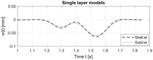
Table 1Comparison of maximal vertical deflection of the slab for shell and solid element models
Shell | Solid | Solid – Shell | % of Shell | |
[s] | 1.541 | 1.544 | + 0.003 | + 0.194 |
[mm] | 0.063 | 0.059 | – 0.004 | – 6.646 |
5. Conclusions
Vehicle-road interaction is the actual engineering problem, solving in many workplaces. The current state of computing technique allows solving the problem in a numerical way in real time. The problem can be modeled using the finite element method in the environment of a commercial software, e.g. ADINA. It is advisable to use the spatial model of vehicle. The road model can be created as a single layer or multilayer model. Single layer models are sufficient in case we want to analyze stress and strain states only in the reinforced concrete slab itself and we are not interested in stress and strain states in the individual subgrade layers. The complexity of the model must be adapted to the quality of the results. Shell elements are preferred in the case if the internal forces are needed to design the structure. The solid elements are advantageous if the output is to be a more detailed analysis of the stress states of the structure. In both cases, the contact forces between the wheel and the road can also be obtained. It is best to combine numerical and experimental procedures together and to verify numerical results. The use of such procedures may have different applications in practice [6-8].
References
-
Edmond N. D., Muho V. Dynamic response of a finite beam resting on a Winkler foundation to a load moving on its surface with variable speed. Soil Dynamics and Earthquake Engineering, Vol. 109, 2018, p. 222-226.
-
Beskou N. D., Theodorakopoulos D. D. Dynamic effects of moving loads on road pavements: a review. Soil Dynamics and Earthquake Engineering, Vol. 31, 2011, p. 547-567.
-
Ducarne L., Ainalis A., Kouroussis G. Assessing the ground vibrations produced by a heavy vehicle traversing a traffic obstacle. Science of The Total Environment, Vol. 612, 2018, p. 1568-1576.
-
ADINA Primer, ADINA System 9.3. ADINA R&D, 2017, www.adina.com.
-
Novotný B., Hanuška A. Theory of Layered Half-Space. VEDA, SAV, Bratislava, 1983, (in Slovak).
-
Kowalska-Koczwara A., et al. Vibration-based damage identification and condition monitoring of metro trains: Warsaw metro case study. Shock and Vibration, Vol. 2018, 2018, p. 8475684.
-
Kotrasová K., Harabinová S., Panulinová E., Kormaníková E. Dynamic response of liquid storage tanks considering soil interaction. Interdisciplinarity in Theory and Practice, Vol. 8, 2015, p. 21-27.
-
Kormaníková E., Kotrasová K. Finite element analysis of damage modeling of fiber reinforced laminate plate. Applied Mechanics and Materials, Vol. 617, 2014, p. 247-252.
About this article

