Abstract
Considering the shortcomings of the traditional energy spectrum algorithm applied to the rolling bearing fault diagnosis, which can only represent the tendency of fault feature transformation with a certain scale, but not adjacent scales contained. In this paper, we propose a fault diagnosis method of rolling bearing based on Support Vector Machine, combining energy spread spectrum and genetic optimization. The extracted signal is denoised and decomposed using wavelet packets, the energy spectrums and energy spread spectrums are calculated based on the decomposed different frequency signal components. The genetic algorithm is used to select the important parameters of the Support Vector Machine and bring the determined parameter values into the Support Vector Machine to generate the GA-SVM model. Then, energy spectrums and energy spread spectrums are inputted into GA-SVM as the characteristic parameters for identification. The experimental results show the two new points of energy spread spectrums and GA-SVM improve the diagnostic rate by up to 28.5 %, it can effectively improve the fault recognition rate of the rolling bearing.
1. Introduction
As an important part of the mechanical equipment, the damage probability of the bearings in the rotating machinery is up to 30 %. In order to improve the production efficiency and reduce the equipment maintenance time and cost, it is necessary to carry on the fault diagnosis and condition monitoring research on the bearing.
At present, the research on fault diagnosis of rolling bearing mainly focuses on the selection and innovation of algorithms such as signal noise reduction, diagnosis and recognition. In signal processing and feature extraction, Abdel-Ouahab Boudraa [1], Danilo P. Mandic [2] and so on applied improved empirical mode decomposition (EMD) to the rolling bearing fault diagnosis noise reduction algorithm. EMD decomposes the signal into a series of IMFs (Intrinsic mode function) components with a characteristic time scale from small to large and high to low frequency and one remainder [3]. The decomposed high-frequency IMFs component of the signal mixed with random noise is usually noisy. After removing the noise IMF component, the fake IMFs component and the remainder, the remaining IMF component is reconstructed, and the newly reconstructed signal is considered to be noise-reduced. But EMD algorithm decomposition process may occur in the phenomenon of aliasing and so on. Yukio Kaneda [4], Chu Fulei [5] applied energy spectrums to the selection of fault characteristic parameters of rolling bearings. Energy spectrum algorithm can only represent a certain frequency range and cannot show the variation trend of the adjacent intervals.
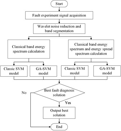
In terms of classification and identification, Fayao Liu [6] and so on applied a state monitoring method based on depth learning theory. Depth learning theory, like artificial neural networks, faces the problem of requiring large amounts of data to train and the difficulty of choosing meta-parameters and network topologies. Since the Support Vector Machine has a large advantage in solving small samples, it has strong ability to improve generalization performance, solve high-dimensional problems and nonlinear problems. In this paper, a rolling bearing fault diagnosis algorithm which combines the energy spread spectrum and the genetic algorithm with the Support Vector Machine is proposed. The genetic algorithm is used to optimize the selection of the Support Vector Machines parameters, which have a great effect on the classification results. The flowchart of the fault diagnosis algorithm in this paper is shown in Fig. 1.
Fig. 1Flowchart of the fault diagnosis algorithm
2. Energy spectrum and energy spread spectrum
According to Parseval’s theorem [7, 8], the signal Fourier transform square is defined as the energy spectrum, which is the signal energy contained in the unit frequency range. Generally, when a transient impact occurs, vibration amplitude changes dramatically and vibration frequency is higher. The instantaneous energy obtained from the original signal after the energy calculation has both kinetic energy and potential energy, so that the transient characteristics of the original signal can be made more obvious [9].
Assuming that the wavelet packet coefficients of the signal decomposed by the -th layer wavelet packet [10] are , ,…, . The corresponding energy of each frequency band is:
The total wavelet packet energy value is:
where is the decomposition level; is the -th band of the -th layer. The article introduces the concept of relative wavelet packet energy and defines the relative wavelet packet energy:
Energy spectrum algorithm can only represent each scale but cannot display the trend of the fault characteristics transformation between adjacent scales. The proposed concept of energy spread spectrums solves this drawback. Energy spread spectrum is defined as the difference between two adjacent energy spectrums, the formula is as follows:
3. Support vector machine and its genetic algorithm optimization
3.1. Support vector machine
Support Vector Machines (SVM) [11, 12], as a machine learning method based on statistical learning theory, can be well used to solve practical problems such as small samples and nonlinearity. The main idea is to establish a classification hyperplane as the decision-making surface, which maximizes the marginalization between positive and negative examples so as to realize the classification of samples. According to literature [13], when the penalty parameter of Support Vector Machine is small, the error is larger and decreases with the increase of , which is an under-learning phenomenon. When is increased gradually, the error is stable at a certain stage. However, when c is too large, the error increases with the increase of , which is an over-learning phenomenon. When the kernel function parameter is small, the training error is small and the testing error is large, which is an over-learning phenomenon. When is large, the training error and the test error are very large, which is an under-learning phenomenon. Therefore, Support Vector Machine , parameter selection is crucial.
3.2. Genetic algorithm optimization support vector machine
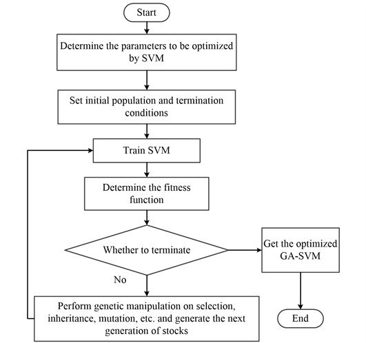
As a classical optimization algorithm, Genetic Algorithm (GA) [14] originally originated from computer simulation of biological systems. In this paper, we choose to optimize the SVM parameters , by GA algorithm to get the best parameters , and bring it into the GA-SVM model. The optimization algorithm flow is shown in Fig. 2.
Fig. 2The flow chart of GA optimized SVM parameters
STEP 1: Initial population generation: The Eq. (5) is used in the paper to construct the initial population to improve the global search ability and avoid the imbalance of distribution in the solution space:
where represents the number of 1 in the generated -th individual (the number of 1 is variable); indicates the lower bound of the number of 1 in the individual, indicates the upper bound of the number of 1 in the individual, and indicates the size of the population. The advantage is that it is easy to search for the best individual when searching.
STEP 2: Regression training is performed on each individual generated by the population, and the mean square error of the cross training is taken as the objective function value, the fitness of each individual is calculated according to Eq. (6):
Among them, the original fitness function is , and the fitness after adjustment is . The value of is determined by the value of , and when is greater than or equal to 1, is a positive integer greater than one; When is less than 1, is a value in (0, 1). and represent the total current evolutionary generation and evolution generation; and respectively represent the best fitness and average fitness of the group.
STEP 3: Select, cross, and mutate operations for trained individuals, get a new generation of evolved individuals and join the next generation of populations. Repeat cross-regression training to calculate the fitness of each individual.
STEP 4: Perform cross-regression training to calculate the fitness of each individual; the iterative algebra reaches the maximum, the algorithm terminates and the optimal parameters under the condition are output; otherwise, it returns to the Step 3 loop execution until the condition is met and the algorithm terminates.
4. Experimental process and results analysis
4.1. Signal denoising and fault frequency analysis
In this paper, the experimental data is selected from Case Western Reserve University of America, in which the sampling frequency is 12000 Hz. Vibration data was collected using accelerometers, which were attached to the housing with magnetic bases. Vibration signals were collected using a 16 channel DAT recorder, digital data was collected at 12,000 samples per second. All data files are in Matlab (*.mat) format. It will be collected in the normal, inner race fault, outer race fault and rolling element fault HP motor bearing original vibration signal and select DDENCMP function to automatically obtain the noisy signal threshold and select “wthresh” function soft threshold denoising. The above original signals are respectively shown in Fig. 3.
Taking the frequency analysis of normal operation state as an example, it can be seen from Fig. 4 that the frequency of the real vibration signal is within the range of 2000 Hz. Therefore, in this paper, a central frequency 1000 Hz of Butterworth low-pass filter was selected. According to reference [15], the frequency extreme values of the four states were all within 500 Hz, so detailed analysis was carried out within the range. It can be seen from the Fig. 5 that the characteristic frequency of inner race fault, outer race fault maximum fault is basically within the theoretical fault characteristic frequency range, and the rolling element fault characteristic frequency is relatively close or even difficult to distinguish. Therefore, the traditional bearing fault characteristic frequency analysis method also has certain deficiencies. The theory characteristic fault frequency of HP motor bearing is shown in Table 1.
Fig. 3The original vibration signals of four states
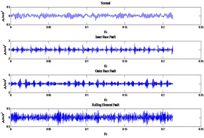
Fig. 4Spectrum diagram of normal operation state
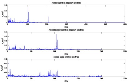
Fig. 5Partial envelope spectrogram of four states
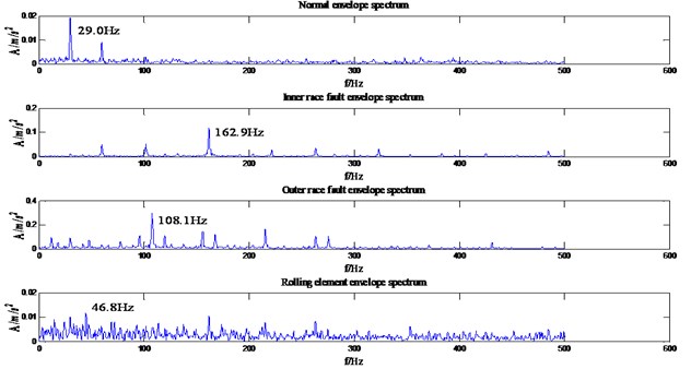
Table 1Frequency table of fault characteristic frequency of the HP motor bearing
Status type | Maximum characteristic frequency |
Inner race fault | 162.1855 Hz |
Outer race fault | 107.3645 Hz |
Rolling element fault | 70.5849 Hz |
4.2. Signal band decomposition and energy feature extraction
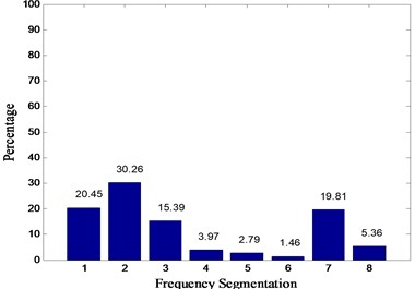
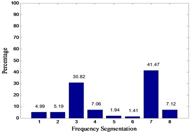
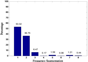
In this paper, Daubechies wavelet is chosen as the wavelet basis function. Among them, db5 wavelets have good regularity, the wavelet coefficients can better represent the characteristics of the original signal. Wavelet packet decomposition of the original signal loss is very small. But with the increase in the number of decomposition layers, the integrity of the information stored will be reduced accordingly. To sum up, in this paper, the signal is decomposed by 3 layers of wavelet packet rely on db5 wavelet basis function and eight different frequency bands are obtained. The relative energy spectrum and energy spread spectrum of eight different frequency bands are calculated respectively as the characteristic parameters according to Eqs. (3) and (4). The typical energy spectrum distribution of the third layer in four states is shown in Fig. 6. As can be seen from the figure, the distinguishing effect of energy spectrum characteristics is obvious, but there is still some similarity between the normal and rolling element fault. The energy spread spectrum can clearly distinguish them in Fig. 7.
Fig. 6Energy spectrum distribution diagrams of four states: a) normal, b) inner race fault, c) outer race fault, d) rolling element fault

a)
b)
c)
d)
4.3. Support vector machine pre-processing based on genetic algorithm optimization
Regarding the optimization of SVM parameters, there is no internationally recognized best method now. The currently used method is to let and take values within a certain range. For the given and , use the training set as the original data set and use the K-CV method to obtain the training set verification classification under this group and . Finally, the accuracy rate is used as the index to select the optimal parameters of the Support Vector Machine and , and the and under the highest accuracy are output. The classic K-CV algorithm divides the raw data into groups (generally average), and each subset data is used as a verification set, and the remaining subset data is used as a training set, so that models are obtained. The average of the classification accuracy of the final verification set of the models is used as the performance index of the classifier under this K-CV.
In the classical K-CV sense, meshing is used to find the best parameters and , although the grid search just can find the local highest classification accuracy. If you want to find the best parameters and in a larger range, it will be time-consuming and computationally intensive. Using genetic algorithm, you can find the global optimal solution without traversing all the parameter points in the grid.
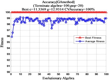
In order to achieve the best Support Vector Machine classification effect, the genetic algorithm is optimized for the and parameters of the Support Vector Machine. This article set the maximum number of iterations maxgen to 200; the largest population sizepop 20; the range of parameters for SVM is [0, 100]; the range of parameters is [0, 200]; and the value for Cross Validation is 5. Finally, the optimized GA-SVM is obtained according to the flow chart in Fig. 1. After optimization by genetic algorithm, 11.3369, 12.9314 is selected from Fig. 8.
Fig. 7The energy spread spectrum of four states
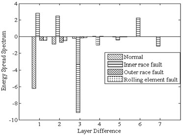
Fig. 8GA optimization c, g parameter results
4.4. The results of GA-SVM classification identification
It will be extracted to the normal, inner race fault, outer race fault and rolling element fault a total of 400 sets of data. In the data of four states, 50 groups were randomly selected as training samples and the remaining 50 groups were input into GA-SVM as testing samples for identification.
Algorithm 4 (a total of 220 sets of data, of which 210 are correctly identified) proposed in this paper is compared with Algorithm 1 (Energy spectrum and normal SVM, a total of 100 sets of data, of which 67 are correctly identified), Algorithm 2 (Energy spectrum and genetic algorithm optimized SVM , a total of 100 sets of data, of which 89 were correctly identified) and Algorithm 3 (Energy spectrum, energy spread spectrum and normal SVM, a total of 100 sets of data, of which 85 were correctly identified). The final recognition result is shown in Table 2 and Fig. 9. (Note: “1” represents normal state, “2” represents inner race fault, “3” represents the outer race fault and “4” represents rolling element fault).
Fig. 9The classification results of four algorithms
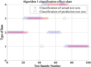
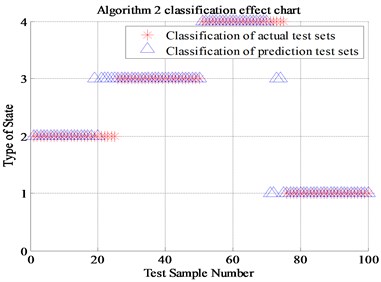
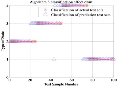
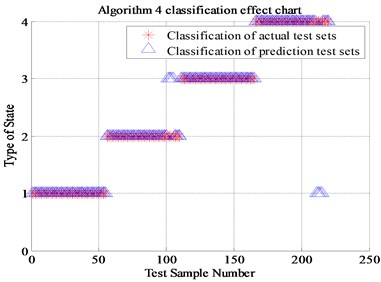
Table 2Comparison of four algorithms recognition rate
Algorithm type | Algorithm recognition rate |
Algorithm 1 (Energy spectrum and normal SVM) | 67 % |
Algorithm 2 (Energy spectrum and GA-SVM) | 89 % |
Algorithm 3 (Energy spread spectrum and normal SVM) | 85 % |
Algorithm 4 (Energy spread spectrum and GA-SVM) | 95.5 % |
It can be seen from Fig. 9, the algorithm 2 compared with the classical algorithm 1, the newly proposed energy spread spectrum concept has improved the fault recognition rate from 67 % to 85 %. The 18 percent fault recognition accuracy improvement results prove that the energy spread spectrum makes up for the regret of energy spectrum, which can only represent each scale but cannot display the trend of the fault characteristics transformation between adjacent scales. The algorithm 3 of genetic algorithm optimized SVM has improved the fault recognition rate from 67 % to 89 % compared with Algorithm 1. The 22 percent fault recognition accuracy proves the significant improvement of genetic algorithm compared with K-CV algorithm. Compared with Algorithm 1, the algorithm 4 that combines energy spread spectrum and genetic algorithm has improved the final fault recognition rate from 67 % to 95.5 %, which is up to 28.5 percentage points. Finally, it can be proved that the newly proposed energy spread spectrum and genetic algorithm for SVM optimization is positive, effective and reasonable in this experiment.
5. Conclusions
Although the classical spectrum analysis or energy spectrum bearing fault diagnosis scheme has certain applications, its diagnostic effect needs to be further improved. By comparing the algorithm 1 (Energy spectrum and normal SVM), the energy spread spectrum and GA-SVM to increase the fault recognition rate by 18 and 22 percentage points respectively, the combination of the two increased by 28.5 percentage points. However, limited to the experimental conditions, this paper focuses on four states detecting under ideal friction and lubrication conditions. In conclusion, it can be proved that the newly proposed energy spread spectrum concept and the optimization of the genetic algorithm are effective and has made a great progress compared with the past. It also has a great reference value for actual mechanical equipment status detection and can be used in the practiced field.
References
-
Abdel-Ouahab Boudra, Jean-Christophe Cexus EMD-Based Signal Filtering. IEEE Transactions on Instrumentation and Measurement, Vol. 56, Issue 6, 2007, p. 2196-2202.
-
Mandic Danilo P., Rehman Naveedur Empirical Mode Decomposition-Based Time-Frequency Analysis of Multivariate Signals: The Power of Adaptive Data Analysis. IEEE Signal Processing Magazine, Vol. 30, Issue 6, 2013, p. 74-86.
-
Bharathi M. R., Mohanty A.R. Underwater sound source localization by EMD-based maximum likelihood method. Acoustics Australia, Vol. 46, Issue 2, 2018, p. 193-203.
-
Kaneda Yukio, Ishihara Takashi Energy dissipation rate and energy spectrum in high resolution direct numerical simulations of turbulence in a periodic box. Physics of Fluids, Vol. 15, Issue 2, 2003, p. 21-24.
-
Fulei Chu, Jin Zhang Extraction of rolling bearing fault feature based on time-wavelet energy spectrum. Journal of Mechanical Engineering, Vol. 17, Issue 47, 2011, p. 44-49.
-
Liu Fayao, Shen Chunhua Learning depth from single monocular images using deep convolutional neural fields. IEEE Transactions on Pattern Analysis and Machine Intelligence, Vol. 38, Issue 10, 2016, p. 2024-2039.
-
Sun Jian, Wang Chenghua Analog circuit fault diagnosis based on wavelet packet energy spectrum and NPE. Chinese Journal of Scientific Instrument, Vol. 9, Issue 24, 2013, p. 2021-2027.
-
Zarei Jafar, Poshtan Javad Bearing fault detection using wavelet packet transform of induction motor stator current. Tribology International, Vol. 40, Issue 2007, 2006, p. 763-769.
-
Eren Levent, Devaney M. J. Bearing damage detection via wavelet packet decomposition of the stator current. IEEE Transactions on Instrumentation and Measurement, Vol. 2, Issue 53, 2004, p. 430-436.
-
Cao Mao-Sen, Ding Yu-Juan Hierarchical wavelet-aided neural intelligent identification of structural damage in noisy conditions. Applied Sciences, Vol. 7, Issue 4, 2017, p. 1-20.
-
Hearst M. A., Dumais S. T. Support vector machines. IEEE Intelligent Systems and their Applications, Vol. 13, Issue 4, 1998, p. 18-28.
-
Tyagi Commander Sunil A comparative study of SVM classifiers and artificial neural networks application for rolling element bearing fault diagnosis using wavelet transform preprocessing. International Journal of Mechanical and Mechatronics Engineering, Vol. 2, Issue 7, 2008, p. 904-912.
-
Yang Shuxia, Wu Jinglong Parameter selection for support vector machines based on genetic algorithms to short-term power load forecasting. Journal of Central South University (Science and Technology), Vol. 1, Issue 40, 2009, p. 180-184.
-
Zhang Yinglu Internet forecasting based on support vector machine optimized by genetic algorithm. Computer Science, Vol. 5, Issue 35, 2008, p. 177-180.
-
Ding Feng, Qin Feng-Wei Application of wavelet denoising and Hilbert transform in fault diagnosis of motor bearing. Electric Machines and Control, Vol. 21, Issue 6, 2017, p. 89-95.
About this article

This research is financially supported by the National Natural Science Foundation of China (Grant No. 51275374).
