Abstract
A novel intelligent fault diagnosis method based on deep learning and particle swarm optimization support vectors machine (PSO-SVM) is proposed. The method uses deep learning neural network (DNN) to extract fault features automatically, and then uses support vector machine to classify diagnose faults based on extracted features. DNN consists of a stack of denoising autoencoders. Through pre-training and fine-tuning of DNN, features of input parameters can be extracted automatically. This paper uses particle swarm optimization algorithm to select the best parameters for SVM. The extracted features from multiple hidden layers of DNN are used as the input of PSO-SVM. Experimental data is derived from the data of rolling bearing test platform of West University. The results demonstrate that deep learning can automatically extract fault feature, which removes the need for manual feature selection, various signal processing technologies and diagnosis experience, and improves the efficiency of fault feature extraction. Under the condition of small sample size, combining the features of the multiple hidden layers as the input into the PSO-SVM can significantly increase the accuracy of fault diagnosis.
1. Introduction
Rotating machinery is one of the most commonly used types of equipment and plays an important role in daily production [1]. In order to improve the productivity and product quality, reduce the cost, the mechanical equipment must be in trouble-free operation. Once a component failure occurs, it will produce a chain reaction, resulting in damage to the equipment. Rotating machinery is key equipment which is widely used in electric power, chemical industry, metallurgy, mining and other industries. If we do not timely diagnose a fault of the rotating machinery, it will cause serious failure of mechanical equipment, resulting in huge economic losses. Therefore, fault diagnosis of the rotating machinery can avoid serious failure, which is of great practical significance to the normal operation of the mechanical equipment [2-4].
The fault identification problem of rotating machinery can be viewed as a classification problem. Under the condition of the same input vectors, a good classifier can be used to effectively judge the fault patterns. The conventional classifiers require a large number of high precision samples, which is not practical. Support vector machine (SVM), developed by Vapnik [5], is a machine learning method based on the statistical learning theory, which solves the problem of ‘over-fitting’, local optimal solution and low convergence rate. Even if the number of samples is small, SVM can still achieve high accuracy and classification results. Some researchers have employed the SVM as a tool for the classification of mechanical faults including bearing [3, 6], gear [7], turbo-pump [8] and induction motor [9]. In the practical application of SVM, an existing problem is how to select the best parameters of SVM. The parameters should be optimized including the penalty parameter and the kernel function parameters . Particle swarm optimization (PSO), proposed by Kennedy and Eberhart [10, 11] and inspired by social behavior of bird flocking or fish schooling is a global optimization technique. Recently, numerous researches on PSO theories or applications have successfully applied PSO to solve multi-dimensional optimization problems [12], artificial network training [13-15], fuzzy system control [16, 17], and so on. Liu, et al. [18] used the multi fault classification algorithm based on wavelet support vector machine (WSVM) to analyze the vibration signals of rolling bearings, and PSO is applied to find the optimal parameters of WSVM. Bao, et al. [19] proposed an efficient memetic algorithm based on PSO and pattern search (PS) for SVM parameter optimization.
Before training by SVM, the features should be extracted from the raw data for classification. Feature extraction aims to extract representative features from the raw signals based on signal processing techniques such as time-domain statistical analysis [20], frequency domain statistical analysis and so on [21, 22]. However, SVM is unable to extract and organize the discriminative information from raw data directly. So, lots of the actual efforts in intelligent diagnosis methods go into the design of feature extraction algorithms in order to obtain the representative features from the signals. Such processes take advantage of human ingenuity but largely rely on prior knowledge about signal processing techniques and diagnostic expertise, which is time-consuming and labor-intensive.
To overcome the weakness, this paper uses the deep learning method to extract the fault feature. Deep learning makes use of artificial neural networks. In 2006, Hinton et al. [23] published an article in the “Science” for the first time, discussed the deep learning theory, and initiated deep learning tide in academia and industry. In recent years, some researchers have applied deep learning in the field of mechanical fault diagnosis, and achieved some results. Samanta et al. [24] utilized time-domain features to characterize the bearing health conditions and employed artificial neural networks (ANNs) and SVM to diagnose faults of bearings. Widodo et al. [25] calculated statistical features from the measured signals and carried out SVM to diagnose the bearing faults. Jia et al. [26] used the deep neural networks to extract fault feature from the massive data. Gan et al. [27] constructed a hierarchical diagnosis network based on deep learning and then applied it in the fault pattern recognition of rolling element bearings. Kim et al. [28] used support vector machines (SVMs) with class probability output networks (CPONs) to provide better generalization power for pattern classification problems.
The quality and quantity of extracted features have a decisive impact on the classification accuracy of SVM. As the deep learning, neural networks have several hidden layers, and each hidden layer represents different features at different levels, this paper proposes a novel method combining the feature of multiple layers as the input into PSO-SVM to improve the classification accuracy of SVM.
The essence of fault diagnosis is feature recognition and classification. This paper presents a method based on deep learning and PSO-SVM for fault intelligent diagnosis. It uses the deep learning neural network to automatically extract the fault feature, and then uses the PSO-SVM to classify the extracted features. The merits of the proposed method are summarized as follows: (1) Deep learning can automatically extract fault features, which removes the need for manual feature selection, various signal processing technologies and diagnosis experience, and improves the efficiency of fault feature extraction. (2) Under the condition of Small size of sample, combining the features of multiple hidden layers as the input of PSO-SVM can significantly increase the accuracy of fault diagnosis.
The rest of this paper is organized as follows: Section 2 briefly introduces the structure and working principle of deep learning neural networks, and presents the SVM and its parameter optimization algorithm PSO. Then, it introduces the procedure of mechanical fault diagnosis method based on deep learning and PSO-SVM. Section 3 validates the effectiveness of the proposed method by using the data of rolling bearing experimental platform of West University. The proposed method is compared with the artificial fault extraction method. In addition, the two methods are compared when small samples and large samples are used for fault diagnosis, as well as when different extracted features are used for diagnosis. Conclusions are drawn in Section 4.
2. Intelligent fault diagnosis method based on Deep learning and PSO-SVM
2.1. Deep learning neural network
2.1.1. Autoencoder, sparse autoencoder and denoising autoencoder
DNN is composed of a plurality of sparse Autoencoders (AE). Autoencoders are a three layer of unsupervised neural network, which is divided into two parts: encoding network and decoding network and the structure is shown in Fig. 1.
Fig. 1Architectural graph of an autoencoder
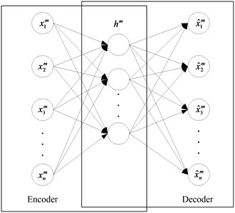
The input and output layers in an autoencoder have the same number of nodes. High dimension of input data can be reduced by encoding network, and reconstructs the coding vector of low dimensional space to the original input data. Because the input signal can be reconstructed in the output layer, the coding vector is a characteristic representation of the input data. Autoencoders should not lose the characteristic information of the input signal as far as possible. In order to realize no losing, the encoder must capture the most important factors which can represent input data. In order to extract the features of input signal without loss of useful information, we introduce the Sparse Autoencoder (SAE). SAE requires that most of the nodes are zero while only a few of the nodes is nonzero (the main character). In order to improve the robustness of the autoencoders, we also introduce the Denoising Autoencoder (DAE). DAE introduces the noise with some statistical characteristics into the sample data, and then codes the sample; the decoding network is estimated in the original form of the sample without noise interference according to the data subject to noise interference. So that DAE can learn from the noisy samples to extract more robust features and reduce the sensitivity of DAE to small random perturbations. The structure of DAE is shown in Fig. 2.
Fig. 2Schematic of a denoising autoencoder
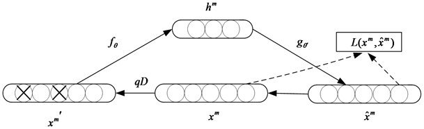
The DAE principle is similar to the human body’s sensory system, such as observing objects. If a small part is covered, people can still identify the object. In the same way, DAE can effectively reduce the influence of random factors on the extraction of health information and improve the robustness of the feature expression by adding noise to the coding and reconstruction. The DNN model which is used in this method is the overlapping sparse denoising autoencoder.
2.1.2. DNN pre-training and fine-tuning
In deep learning, DNN is first trained by the unsupervised method, which can help the DNN to capture the fault characteristics of the input signal effectively. Then, DNN is adjusted by the supervised learning method to optimize the expression of DNN on the fault characteristics. This paper uses denoising autoencoder as a non unsupervised algorithm for pre-training, and uses the BP algorithm as the supervised algorithm for fine-tuning stage.
Pre-training is an unsupervised learning from bottom to top. First, the first layer is trained with the training sample data, and the connection weights and the bias parameters of the first layer are obtained. By the principle of denoising autoencoder, DAE model can learn the structure of the data itself and identify the characteristics of the input. The output of the first layer is used as the input of the second layer. Train the second layer to get connection weights and bias parameters of the second layer. And then layer by layer. The final features are reconstructed based on the learning of multiple layers. As shown in Fig. 3, given a label free training sample set , the coding network transforms each training sample to the coding vector by the coding function :
where is the activation function of the coded network; and is the parameter set for the coded network, and ; where and , respectively, are the connection weights and bias parameters of the coding network; DAE completes the training of the whole network by minimizing the reconstruction error between and :
Fig. 3The pre-training and fine-tuning of the DNN
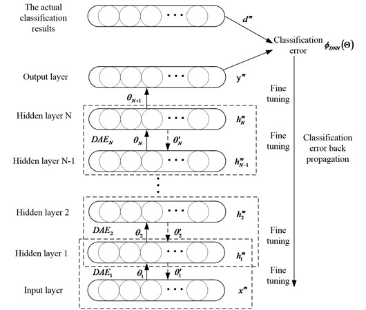
Fine-tuning is supervised learning from top to bottom. With the labeled training data, the error transports from top to bottom to fine tune the deep neural network. This process is a supervised training process. Specific as shown in Fig. 3, this method uses the BP algorithm to fine tune the DNN parameters. The output of DNN is expressed as:
where is the parameter of the output layer.
Assume that of the health condition type is , DNN is fine-tuned by minimizing the :
where is the function of minimizing the error between and ; where is the parameter set of DNN, and .
2.2. PSO-SVM
2.2.1. Support vector machine
The support vector machine based on statistical learning theory proposed by Vapnik et al. [5] is a better method to realize the structural risk minimization principle, which provides a new way of thinking to solve the small sample size classification, nonlinear problem.
The basic idea of SVM is to increase dimension and linearization: define the optimal linear hyper plane, and reduce the algorithm of finding the optimal linear hyper plane to a convex programming problem. Then, based on the Mercer kernel expansion law, the sample space is mapped to a high dimensional and even infinite dimensional feature space by nonlinear mapping, so as to the linear learning machine can be used in the feature space to solve the problem of highly nonlinear classification and regression in the sample space.
Suppose a training set with samples , , can be separated by a super plane without errors, and the distance between the nearest vector and the hyper plane is the largest, which is called the optimal hyper plane, as shown in Fig. 4.
Fig. 4Optimal hyper plane of the support vector machine
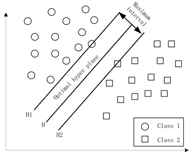
Define two standard hyper planes and , where and are over all samples from the nearest classification and parallel to the plane of the classification of hyper plane, the distance between them is .
The maximum interval is equal to the minimum value . Taking into account the correct classification of all training samples, the following should be satisfied:
Two can be combined into:
Therefore, the purpose of the support vector machine is to use the following formula to construct the classified hyper plane to classify all the samples correctly:
Because the objective function and the constraint condition are convex, according to the optimization theory, this problem has a unique global minimum solution. Applying Lagrange multipliers and taking into account the KKT condition:
The optimal hyper plane decision function can be obtained:
For linear separable case, by introducing slack variables , modifying the objective function and constraints, and then solving the method completely with similar application, we get:
If the training data can’t be separated, maximizing the class interval hyper plane requires eliminating those misclassified samples.
In the nonlinear case, the support vector machine uses the nonlinear mapping algorithm in the feature space, that is, the input vector is mapped to a high dimensional feature space by the prior selection of a certain nonlinear mapping., . Then in the high dimension space using linear support vector machine to classify. The objective function and constraint conditions are:
Then the classification decision function is obtained:
For nonlinear classification problems, the core idea is to increase the linear spatial dimensions, namely the data sample low-dimensional space is transformed into a high-dimensional space via a mapping function, and thus the nonlinear classification problem is converted to a linear classification problem. Linear classification of samples in high dimensional Hilbert space is carried out to obtain the optimal classification hyper plane and decision function to return to low dimensional space.
2.2.2. Particle swarm optimization
SVM kernel function parameter g and parameter c have a major impact on its classification accuracy. So, in this paper, particle swarm optimization algorithm is used to optimize the parameters of SVM. In this way, we can effectively prevent the low classification accuracy due to the lack of experience in constructing kernel function parameters and penalty factors.
Particle swarm optimization algorithm was first proposed by J. Kennedy and R. C. Eberhart based on swarm intelligence theory in 1995 [10]. It’s mathematical expression is as follows: Assuming that in a dimensional optimization space, there are a group of particles, speed of the th particles can be expressed as , its position can be expressed as the optimal position of the current search for the particle is , and the optimal position of the whole population is , the particle swarm updating equation is as follows:
If , .
If , .
; , where is the current iteration number, and are the acceleration constant, and are random numbers between [0, 1], and is the inertia weight.
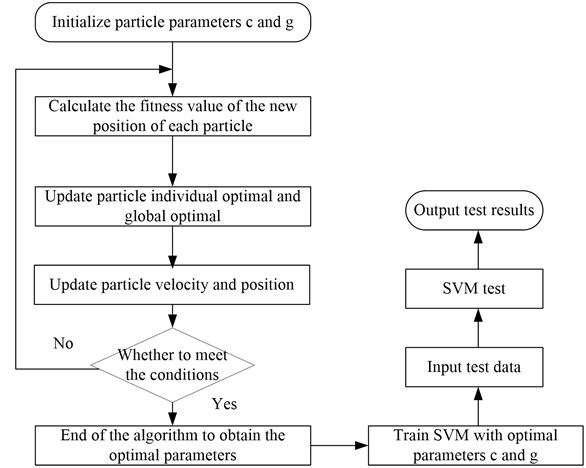
The PSO algorithm is used to optimize the parameters of SVM, and the specific steps are shown in Fig. 5.
Fig. 5Flowchart of PSO algorithm to optimize the parameters of SVM
2.3. Fault diagnosis model based on deep learning and PSO-SVM
The spectral signal of the mechanical vibration signal works as the input layer, and multiple DAEs are stacked together to form DNN. The output of the first level DAE is the second level DAE input, the output of the second level DAE is the third level DAE input, and so on. In this method, the output of the last hidden layer or the last multiple hidden layers is used as the input of the PSO-SVM. PSO-SVM classifies the features which are extracted by the deep learning to complete the fault diagnosis.
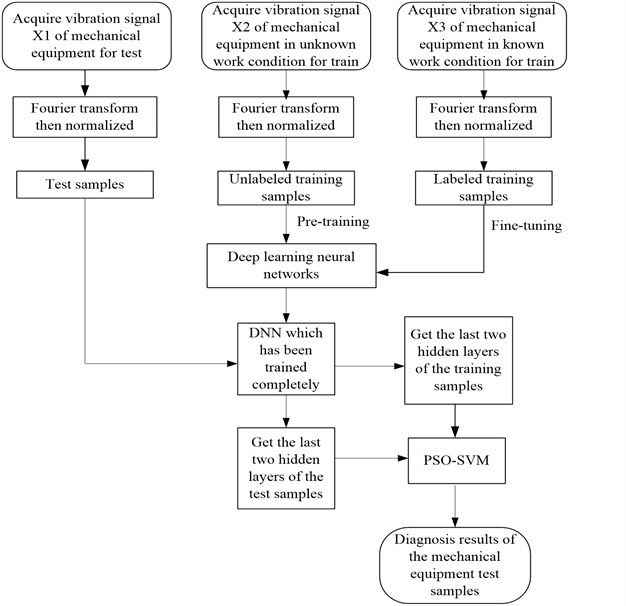
A method for mechanical fault diagnosis based on deep learning and PSO-SVM comprises the following steps:
Step 1: The original vibration data of mechanical equipment is used as the input sample, and then the fast Fourier transform is applied to get a new input sample spectrum signal .
Step 2: By means of the linear normalization method, the vibration spectrum signal is obtained by normalizing the vibration spectrum signal .
Linear normalization method: .
Step 3: Put bearing vibration spectrum signal into the DNN, then use the DNN to extract features from the signal .
Step 4: Put the features which are extracted from DNN into the SVM, and then use the particle swarm optimization algorithm to optimize the support vector machine parameters. After training, put the testing date into the SVM. Finally, we can get the diagnosis results of the mechanical equipment.
Fig. 6Flowchart of fault diagnosis method for mechanical equipment based on deep learning and support vector machine
DNN’s pre-training begins from the bottom, layer by layer to the top. This is the biggest difference with the traditional neural network, so as to avoid the neural network into the local optimal solution. DNN’s fine-tuning is through training the labeled data and use top-down error transmission error, so that the neural network parameters are closer to the global optimum, which can achieve better results.
3. Fault diagnosis using the proposed method
3.1. Experimental configurations
As shown in Fig. 7 and Fig. 8, the test platform consists of a 2 hp motor (left), a torque transducer/encoder (center), a load motor (right). The test platform bearing comprises a drive end bearing and a fan end bearing. The acceleration sensors are respectively arranged at the driving end of the motor casing and the fan end, at the position of 12 o’clock. The vibration signal is collected by a 16-channel DAT recorder, and the drive end bearing fault data sampling frequency is 48000 samples per second. In this experiment, we select the drive end bearing as the research object. Data are collected when the motor load is 3 HP, and the drive end bearing has different fault conditions: normal, inner fault, outer race fault and rolling body fault. Three fault degrees are used for the fault of the inner ring, the outer ring and the rolling body: 0.007, 0.014, 0.021. Single point faults were introduced to the test bearings using electro-discharge machining with fault diameters of 7 mils, 14 mils, 21 mils (1 mil = 0.001 inches). And fault diameters of 7 mils, 14 mils, 21 mils corresponding to the light, medium and heavy fault level. So, this test has ten different working conditions. For each working condition, we divide the collected data into 120 samples and each sample has 4000 sample points. For each working condition, we randomly select 60 groups of samples as the training samples, and use the remaining 60 groups of samples as test samples. Table 1 summarizes the different fault degrees as follows.
Fig. 7Rolling bearing test platform of West University
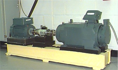
Fig. 8Sketch of the rolling bearing test platform
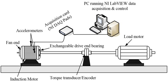
Table 1The detail lists of the test and training samples
Fault type | Fault level | Training/test sample | Data file | Classification label |
Normal | 0 | 60/60 | 100DE | 1 |
Inner ring fault | 0.007 | 60/60 | 112DE | 2 |
Inner ring fault | 0.014 | 60/60 | 177DE | 3 |
Inner ring fault | 0.021 | 60/60 | 217DE | 4 |
Outer ring fault | 0.007 | 60/60 | 138DE | 5 |
Outer ring fault | 0.014 | 60/60 | 204DE | 6 |
Outer ring fault | 0.021 | 60/60 | 241DE | 7 |
Rolling element fault | 0.007 | 60/60 | 125DE | 8 |
Rolling element fault | 0.014 | 60/60 | 192DE | 9 |
Rolling element fault | 0.021 | 60/60 | 229DE | 10 |
3.2. Pre- training and fine-tuning of DNN
The vibration signals are divided into training samples and testing samples randomly. Then the selected sample is analyzed by fast Fourier algorithm. The time domain sampling number of each sample is 4000. While the spectrum of Fourier transform is symmetrical, we take the first 2000 sampling points of the spectrum as the spectral signal . Then linear normalization method is used to get the new spectrum signal . Normalization is not only able to improve the deep learning classification accuracy, but also can reduce the classification computation time. The number of the input layer of the DNN is determined to be 2000. In this paper, the network structure of DNN is set to 2000-500-300-200-10, and the output layer is determined by the classification tag. In addition, in order to enhance the robustness of fault diagnosis, noise encoding network will contain certain statistical properties to sample data.
3.3. Parameter optimization process of particle swarm optimization algorithm
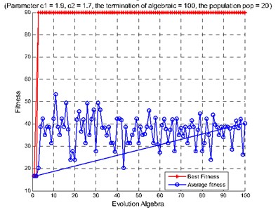
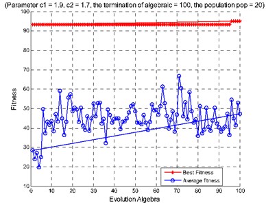
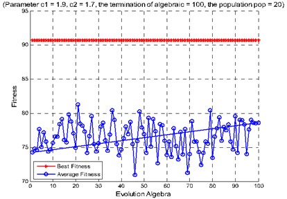
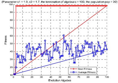
The particle swarm optimization algorithm is set to the maximum number of evolution for 100. The population particle number is 20. The learning factor is 1.9 and the learning factor is 1.7. The parameter 0.4 and the velocity in the velocity update formula in front of the elastic coefficient is 1. The SVM Cross Validation parameter 3, the range of is [0, 1, 200] and the range of parameters for g is [0.01, 1000]. An average relative error of support vector machine is used as fitness function. After optimizing through the particle swarm optimization algorithm, the parameters of and are obtained, and the prediction model of support vector machine is determined.
3.4. Test results for PSO-SVM
The 600 rolling bearings test samples are selected randomly as training samples for SVM and the rest samples are used as testing samples for SVM. Using the proposed method for fault diagnosis, when the second hidden layer is used as the support vector machine input parameters, its recognition accuracy rate is 98.5 %; When the third hidden layer is used as the support vector machine input parameters, its recognition accuracy rate is 98.333 %; When the second hidden layer and the third hidden layer are used as the support vector machine input parameters, its recognition accuracy rate is 98.667 %, as shown in Fig. 9. In addition, we test the method using reduced training and testing samples (60 each). When the second hidden layer is used as the support vector machine input parameters, its recognition accuracy rate is 90 %; When the third hidden layer is used as the support vector machine input parameters, its recognition accuracy rate is 83.33 %; When the second hidden layer and the third hidden layer are used as the support vector machine input parameters, its recognition accuracy rate is 95 %, as shown in Fig. 11. The above experiments show that, under the condition of small samples, the features of the two hidden layer can be used as the input of support vector machine to significantly improve the accuracy of fault diagnosis. Table 2 is accuracies of different input parameters and their corresponding SVM classification under big sample conditions. Table 3 is accuracies of different input parameters and their corresponding SVM classification under small sample conditions.
Fig. 9Diagnosis results of rolling bearing large samples: a) features extracted from the second hidden layer as the input, b) features extracted from the third hidden layer as the input, c) features extracted from the second and the third hidden layers as the input
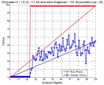
a)
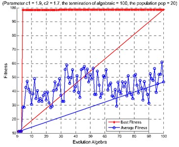
b)
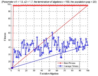
c)
Table 2Large samples: different input parameters and their corresponding SVM classification accuracy
Input parameters | SVM classification accuracy |
Features extracted from the second hidden layer | 98.500 % (591/600) |
Features extracted from the third hidden layer | 98.333 % (590/600) |
Features extracted from the second and third hidden layer | 98.667 % (592/600) |
Table 3Small samples: different input parameters and their corresponding SVM classification accuracy
Input parameters | SVM classification accuracy |
Features extracted from the second hidden layer | 90.00 % (54/60) |
Features extracted from the third hidden layer | 83.33 % (50/60) |
Features extracted from the second and third hidden layer | 95.00 % (57/60) |
We also compare the proposed method with the traditional method. The traditional method combines artificial feature extraction with PSO-SVM for diagnosis. Firstly, commonly used frequency-domain diagnostic features are extracted from the vibration signals obtained from the rolling bearing test platform. Here are the frequency-domain extracted features by artificial means, absolute mean amplitude, RMS, peak, peak to peak, shape factor, crest factor, impulse indicator, margin indicator and kurtosis indicator and so on [20-22]. These feature parameters represent the fault types of vibration signals. As shown in Table 1, the traditional method and the proposed method both use the 600 training samples, which are randomly selected, for SVM to train, and both use the remaining 600 test samples for SVM to test. SVM uses the radial basis kernel function, the kernel function parameters and penalty factors are obtained by the particle swarm algorithm. The difference is that the mentioned method uses DNN to extract features, and the traditional method uses artificial methods to extract features. As shown in Fig. 10, compared with the method based on the combination of the artificially extracted features and the PSO-SVM, the proposed method has higher accuracy of fault diagnosis.
Fig. 10Diagnosis results of rolling bearing small samples: a) features extracted from the second hidden layer as the input, b) features extracted from the third hidden layer as the input, c) features extracted from the second and the third hidden layers as the input
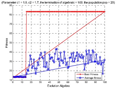
a)
b)
c)
One of basic reasons for high accuracy of the proposed method is that the method can be used to extract fault features from vibration spectrum adaptively. In order to verify the feature extraction capabilities of the proposed method, principal component analysis is used to identify the first three principal components of extracted features from both the proposed method and the traditional method. “First PC” means first principal components; “Second PC” means second principal components; “Third PC” means third principal components. Fig. 12(a) is the scatter plots of principal components for the artificially extracted features. We can see each condition scatter intertwined, showing there is no regular accumulation mode and indicating that the ability of artificially extracting fault feature is weak. Fig. 12(b) is the Scatter plots of principal components for the learned features. Compared with Fig. 12(a), we can see that the scattered points of most conditions are collected together, and the points are effectively separated. These results indicate that deep learning method can extract fault features from vibration spectrum adaptively. Compared with artificially extracted fault features, it not only saves a lot of time and manpower, but also improves the accuracy of diagnosis.
Fig. 11Diagnosis accuracy rate of rolling bearing: a) use the method of combining artificial extracted feature and PSO-SVM, b) use the method of combining deep learning and PSO-SVM
a)
b)
Fig. 12Scatter plots of principal components: a) use artificial extracted features, b) use learned features
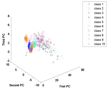
a)
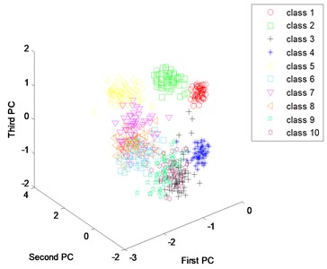
b)
4. Conclusions
In summary, an intelligent fault diagnosis method is proposed based on the deep learning neural network and particle swarm optimization support vector machine. The frequency domain statistical features are extracted by using the artificial method and deep learning method respectively. And then the extracted feature principal component is analyzed. The results show that the fault feature extracted by deep learning has better distinguishably, and it is more suitable for subsequent intelligent classification and fault diagnosis. In conclusion, the DNN network can extract the essential features of the input data automatically. So, it can automatically dig out rich information which is hidden in the data, avoid the need for prior diagnosis experience and signal processing technologies, and improve the efficiency of fault feature extraction. With the extracted features from two layers of the deep learning algorithm, we use particle swarm optimization algorithm to optimize the parameters of support vector machine, and then use support vector machine to diagnose the fault of rolling bearing. Those steps effectively improve the accuracy of rolling bearing fault diagnosis. This method is of great significance to the intelligent fault diagnosis.
References
-
Xue H., Wang H., Chen P. Automatic diagnosis method for structural fault of rotating machinery based on distinctive frequency components and support vector machines under varied operating conditions. Neurocomputing, Vol. 116, 2013, p. 326-335.
-
Lei Y., He Z., Zi Y. Fault diagnosis of rotating machinery based on multiple ANFIS combination with Gas. Mechanical Systems and Signal Processing, Vol. 21, 2007, p. 2280-2294.
-
Konar P., Chattopadhyay P. Bearing fault detection of induction motor using wavelet and Support Vector Machines (SVMs). Applied Soft Computing, Vol. 11, 2011, p. 4203-4211.
-
Mogal S. P., Lalwani D. I. Experimental investigation of unbalance and misalignment in rotor bearing system using order analysis. Journal of Measurements in Engineering, Vol. 3, Issue 4, 2015, p. 114-122.
-
Mercer J. Functions of positive and negative type and their connection with the theory of integral equation. Philosophical Transactions of the Royal Society of London, Vol. 209, 1999, p. 415-446.
-
Abbasion S., Rafsanjani A., Farshidianfar A., et al. Rolling element bearings multi-fault classification based on the wavelet denoising and support vector machine. Mechanical Systems and Signal Processing, Vol. 21, 2007, p. 2933-2945.
-
Samanta B. Gear fault detection using artificial neural networks and support vector machines with genetic algorithms. Mechanical Systems and Signal Processing, Vol. 18, Issue 3, 2004, p. 625-644.
-
Yuan S., Chu F. Support vector machines-based fault diagnosis for turbo-pump rotor. Mechanical Systems and Signal Processing, Vol. 20, Issue 4, 2006, p. 939-952.
-
Yang B., Han T., Hwang W. Fault diagnosis of rotating machinery based on multi-class support vector machines. Journal of Mechanical Science and Technology, Vol. 19, 2005, p. 845-858.
-
Kennedy J., Eberhart R. C. Particle swarm optimization. Proceedings of IEEE International Conference on Neural Networks, Piscataway, NJ, Vol. 4, 1995, p. 1942-1948.
-
Kennedy J., Eberhart R. C., Shi Y. Swarm Intelligence. Morgan Kaufmann Publishers Inc., San Francisco, CA, 2001, p. 475-495.
-
Brits R., Engelbrecht A. P., Bergh F. Locating multiple optima using particle swarm optimization. Applied Mathematics and Computation, Vol. 189, Issue 2, 2007, p. 1859-1883.
-
Geethanjali M., Slochanal S. M. R., Bhavani R. PSO trained ANN-based differential protection scheme for power transformers. Neurocomputing, Vol. 71, 2008, p. 904-918.
-
Che Z. H. PSO-based back-propagation artificial neural network for product and mold cost estimation of plastic injection molding. Computers and Industrial Engineering, Vol. 58, 2010, p. 625-637.
-
Yi D., Ge X. An improved PSO-based ANN with simulated annealing technique. Neurocomputing, Vol. 63, 2005, p. 527-533.
-
Bingul Z., Karahan O. A fuzzy logic controller tuned with PSO for 2 DOF robot trajectory control. Expert Systems with Applications, Vol. 38, Issue 1, 2011, p. 1017-1031.
-
Marinaki M., Marinakis Y., Stavroulakis G. E. Fuzzy control optimized by PSO for vibration suppression of beams. Control Engineering Practice, Vol. 18, Issue 6, 2010, p. 618-629.
-
Liu Z., Cao H., Chen X., Multi -fault classification based on wavelet SVM with PSO algorithm to analyze vibration signals from rolling element bearings. Neurocomputing, Vol. 99, Issue 1, 2013, p. 399-410.
-
Bao Y., Z. H., Xiong T. A PSO and pattern search based memetic algorithm for SVMs parameters optimization. Neurocomputing, Vol. 117, Issue 6, 2014, p. 98-106.
-
Lei Y., Zuo M. J., He Z., Zi Y. A multidimensional hybrid intelligent method for gear fault diagnosis, Expert Systems with Applications, Vol. 37, Issue 2, 2010, p. 1419-1430.
-
Kankar P. K., Sharma S. C., Harsha S. P. Fault diagnosis of ball bearings using machine learning methods. Expert Systems with Applications, Vol. 38, Issue 3, 2011, p. 1876-1886.
-
Li W., Tsai Y. P., Chiu C. L. The experimental study of the expert system for diagnosing unbalances by ANN and acoustic signals. Journal of Sound and Vibration, Vol. 272, Issues 1-2, 2004, p. 69-83.
-
Hinton G. E., Osindero S., Teh Y. W. A fast learning algorithm for deep belief nets. Neural Computing, Vol. 18, Issue 7, 2006, p. 1527-54.
-
Samanta B., Nataraj C. Use of particle swarm optimization for machinery fault detection. Engineering Applications of Artificial Intelligence, Vol. 22, Issue 2, 2009, p. 308-316.
-
Widodo A., Kim E. Y., Son J. D. Fault diagnosis of low speed bearing based on relevance vector machine and support vector machine. Expert Systems with Applications, Vol. 36, Issue 3, 2009, p. 7252-7261.
-
Jia F., Lei Y., Lin J. Deep neural networks: A promising tool for fault characteristic mining and intelligent diagnosis of rotating machinery with massive data. Mechanical Systems and Signal Processing, Vol. 72, 2015, p. 303-315.
-
Gan M., Wang C., Zhu C. Construction of hierarchical diagnosis network based on deep learning and its application in the fault pattern recognition of rolling element bearings. Mechanical Systems and Signal Processing, Vol. 72, 2016, p. 92-104.
-
Kim S., Yu Z., Kil R. M., Lee M. Deep learning of support vector machines with class probability output networks. Neural Networks, Vol. 64, 2015, p. 19-28.
Cited by
About this article

This work was supported by the National Natural Science Foundation of China (Grant No. 51475407), Hebei Provincial Natural Science Foundation of China (No. E2015203190), and Key Project of Natural Science Research in Colleges and Universities of Hebei Province (Grant No. ZD2015050).
