Abstract
In this paper, a multi span concrete girder highway bridge with a 60 degree skewness is used for developing seismic analytical fragility curves for different performance level of the bridge. A detailed finite element modeling of the bridge is presented. Incremental dynamic analysis (IDA) is applied to the bridge in longitudinal direction of the bridge to capture the seismic response of the bridge incrementally. A suite of 14 earthquake ground motions with different range of PGAs are used in nonlinear dynamic analysis of the bridge. Different spectral intensity measures and PGA are studied to find the proficient intensity measure to figure out the analytical fragility curves. The results show that the Sa (1.2 T1,5 %) is the most proficient intensity measure for the current study.
1. Introduction
An earthquake is a random phenomenon, and its prediction is impossible. There are two types of uncertainties; one is related to the structural components and the other one is related to the earthquake itself. One of the approaches that considers both of them simultaneously is probabilistic framework. Thus, the goals of Performance Earthquake Engineering Research center (PEER) are: 1) to define a structural response parameter () such as the drift ratio and a threshold () for it 2) to evaluate the mean annual rate of the occurrences characterized by a level of () greater than () 3) to calculate, based on , the probability to overcome the threshold () in a year [1]. With a calculating the probability that the structure during its useful life (50 years) experiences a certain level of response is simply possible. Therefore, the calculation can be considered as a criterion of the seismic performance of the structure. The direct method of calculating the structural response recording in a time interval, is long enough. For simplicity, assume that the response variable maximum is relative to deformation classes. The direct calculation of the structural response to a prolonged period of time is recorded and the number of each response values plotted. If the frequency is equal to the number of observed when calculating the average rate of annual cumulative cross- over function would not be very difficult [1].
Systematic decision making in the field of earthquake mitigation is required by a quantitative assessment of risk structures. Pacific Earthquake Engineering Research Center (PEER), codified a method to solve the probabilistic response of structures. To better describing the vulnerable condition in a bridge or structures is using fragility functions or vulnerability functions. Vulnerability functions gives the probability of the losses given a level of ground motion and the fragility functions gives the probability of exceeding different limit states (such as damage or injury levels) given a level of ground motions. Fragility curves are one of the important procedures of seismic risk assessment. They relate the seismic intensity to the probability of reaching or exceeding a level of damage (e.g. minor, moderate, extensive, collapse) for each element at risk. The level of earthquake can be quantified using different earthquake intensity parameters, including peak ground acceleration/velocity/displacement, spectral acceleration, spectral velocity or spectral displacement. They are often described by a lognormal probability distribution function. There are several approaches can be used to establish the fragility curves. They can be grouped under empirical, judgmental, analytical and hybrid. Empirical methods are based on past earthquake surveys. The empirical curves are specific to a particular site because they are derived from specific seismo-tectonic and geotechnical conditions and properties of the damaged structures. Judgment fragility curves are based on expert opinion and experience. The other limitations on the empirical fragility curves are having a not sufficient and reliable post-earthquake damage data. Therefore, they are versatile and relatively fast to derive, but their reliability is questionable because of their dependence on the experiences of the experts consulted. Analytical fragility curves adopt damage distributions simulated from the analyses of structural models under increasing earthquake loads as their statistical basis. Analyses can result in a reduced bias and increased reliability of the vulnerability estimates for different structures compared to expert opinion. Analytical approaches are becoming ever more attractive in terms of the ease and efficiency by which data can be generated [2].
A statistical analysis approach has been used to calculate the fragility of bridges subjected to several recent earthquakes [3-5].
There is no other way to prepare fragility curves of Highway Bridges with no data on the actual bridge damage and ground motion data unless using analytical methods. Analytical fragility curves are developed either through nonlinear static analysis and nonlinear time history analysis [6-13]. The procedure to develop fragility curves using nonlinear time history analysis is shown in Fig. 1 [14].
Fig. 1Analytical fragility curve generation using non-linear time history analysis [14]
![Analytical fragility curve generation using non-linear time history analysis [14]](https://static-01.extrica.com/articles/18340/18340-img1.jpg)
In this paper, incremental dynamic (IDA) analysis is used to develop seismic analytical fragility functions of the bridge. The main objective of this research is to determine the vulnerability of a multi-span skewed concrete girder highway bridge when subjected to a medium to strong earthquake.
2. Configuration of the bridge
The bridge model used in this paper is derived from the non-skewed model developed by Nielson [14]. Fig. 2 is shown the width of the bride (15.1 m) and the height of the piers (4.6 m). Total length of the bridge is 48.8 m and its three spans have 12.2-24.4 and 12.2 m length. The bridge has eight AASHTO type prestressed girders. AASHTO Type I and III girders are used for the end and center spans. The pads for end spans are 406 mm long by 152 mm wide and 25.4 mm thick and for the center span which are 559 mm long by 203 mm wide and still 25.4 mm thick. The concrete strength at the design procedure is assumed to be 20.7 MPa while the yield strength of reinforcing steel is 414 MPa. More detailed specifications of these columns are in an investigation of existing bridge plans and also from the work done by Hwang et al. [7]. Fig. 2 shows the column section and the bridge.
Fig. 2General elevation and concrete member reinforcing layout; deck detail; column [14]
![General elevation and concrete member reinforcing layout; deck detail; column [14]](https://static-01.extrica.com/articles/18340/18340-img2.jpg)
![General elevation and concrete member reinforcing layout; deck detail; column [14]](https://static-01.extrica.com/articles/18340/18340-img3.jpg)
![General elevation and concrete member reinforcing layout; deck detail; column [14]](https://static-01.extrica.com/articles/18340/18340-img4.jpg)
![General elevation and concrete member reinforcing layout; deck detail; column [14]](https://static-01.extrica.com/articles/18340/18340-img5.jpg)
2.1. Bridge modelling description
The bridge has been modelled with different linear and nonlinear elements. The elements used for bridge modelling are as follow:
a) FRAME element:
1. Linear frame elements used for modelling of the pre-stressed concrete girders and cap beams.
2. Nonlinear-Frame elements used for modeling the real behavior of the columns in the bridge. Each column divided to 10 equal parts for better capturing their behavior. The nonlinearity in their frame elements were assigned to the to the top and bottom of the column because of the high probable place of the plastic hinges.
b) SHELL elements:
1. To combine the membrane and the plate behavior are using shell elements. Each joint in a shell object has 6 degree of freedom and the frame objects are having 6 degree of freedom. The deck of the bridge used shell elements with the small size of the mesh which is about 1 m×0.5 m.
c) LINK elements:
1. To model the linear behavior of the elastic bearing, a linear link elements were used. The bearing is resting between the girders and cap beams. Two joint linear link elements to use for the modelling in side-span and mide-spans bearing. One joint linear link elements were used for the modeling of the abutments at the ends.
d) FIBER hinges:
1. To define the coupled axial and biaxial-bending behavior in frame objects and distributed plasticity along structural element, the fiber hinges are used. The cross section of the bridge columns are discretized into a series of representative axial fibers which extend longitudinally along hinge length. The scheme of the discretized section is shown in Fig. 3. In this model, the structural element is divided in three types of fibers: some fibers are used for modeling of longitudinal steel reinforcing bars; some of fibers are used to define nonlinear behavior of confined concrete which consists of core concrete; and other fibers are defined for unconfined concrete which includes cover concrete. Also, for each fiber, the stress/strain field is determined. fiber hinges models have been considered: 1) Mander model [15] has been adopted for confined and un-confined concrete 2) typical steel stress-strain (Elasto-plastic) model with no hardening has been adopted for concrete reinforcement.
A rigid bar is used to connect the nodes between girders and bearings, bearings and cap beams, and cap beams and tops of the columns. Abutments and the column boundary conditions are fixed-free in the longitudinal direction and fixed-fixed in the transverse direction. In the longitudinal direction, each column acts as a vertical cantilever beam therefore the longitudinal motion of the bridge is the most critical response which could cause damage to bridge components. The bearings of centre spans have an initial stiffness of 6.2 kN/mm and the end spans have an initial stiffness of 3.4 kN/mm.
Fig. 3Distribution of fibers in circular section [15]
![Distribution of fibers in circular section [15]](https://static-01.extrica.com/articles/18340/18340-img6.jpg)
3. Seismic ground motion records
FEMA-P695 [16] is suggested a suite numbers of earthquake ground motion which has been selected from a great various record selection procedure. Table 1, shows the same information of 14 earthquake ground motion records with different range of PGA form medium to strong motions which are used to perform incremental dynamic analysis (IDA).
4. Incremental dynamic analysis (IDA)
Incremental dynamic analysis (IDA) is one of the effective approaches to define the linear and nonlinear behavior of the bridge. In this approach, the earthquake ground motions are scaled to the PGA 1 g and applied to the bridge with increment of 0.1 g [16]. In each step, a full nonlinear time history analysis is done and the nonlinear response of the structure is captured. Different intensity measures were suggested to consider in IDA analysis. In this study, PGA and ten spectral intensity measures are used.
Table 1Characteristics of the earthquake ground motion histories [16]
Earthquake | Recording station | |||||
ID No. | M | PGA (g) | Year | Name | Name | Owner |
1 | 7.0 | 0.48 | 1992 | Cape Mendocino | Rio Dell Overpass | USGS |
2 | 7.6 | 0.21 | 1999 | Chi-Chi, Taiwan | CHY101 | CWB |
3 | 7.1 | 0.82 | 1999 | Duzce, Turkey | Bolu | ERD |
4 | 6.5 | 0.45 | 1976 | Friuli, Italy | Tolmezzo | – |
5 | 7.1 | 0.35 | 1999 | Hector Mine | Hector | SCSN |
6 | 6.5 | 0.34 | 1979 | Imperial Valley | Delt | UNAMUCSD |
7 | 6.9 | 0.38 | 1995 | Kobe, Japan | Nishi-Akashi | CUE |
8 | 7.5 | 0.24 | 1999 | Kokaeli, Turkey | Duzce | ERD |
9 | 7.3 | 0.36 | 1992 | Landers | Yemo Fire Station | CDMG |
10 | 6.9 | 0.42 | 1989 | Loma Prieta | Capitola | CDMG |
11 | 7.4 | 0.56 | 1990 | Manjil | Abbar | BHRC |
12 | 6.7 | 0.55 | 1994 | Northridge | Beverly Hills-Mulhol | USC |
13 | 6.6 | 0.36 | 1971 | San Ferando | LA-Hollywood Stor | CDMG |
14 | 6.5 | 0.51 | 1987 | Superstition Hills | El Centro Imp. Co | CDMG |
5. Intensity measures and fragility curves
Fragility curves were formulated by the work presented by Cornell et al. [17] condition upon an Intensity Measure (IM). The fragility curves are the relation between the seismic hazard and response of structures and modeled as lognormal distribution Cornell et al. [17]:
where is standard normal cumulative distribution function, is median value of the structural demand in terms of a seismic intensity, is logarithmic standard deviation, or dispersion, of the demand conditioned on the IM.
The relation between SD and IM estimated as:
With a linear regression, we can obtain the coefficient of a and b and re-written the Eq. (5) as:
The dispersion of the mean demand conditioned on the IM is:
where is number of ground motions, is peak demands.
5.1. Efficient intensity measure
If an IM is efficient it should have a less dispersion about the median of the results of nonlinear time history analysis. is the dispersion of the results around the median of the response in this study. The lower values of leads to a more efficient intensity measure Padgett et al. [18].
5.2. Practical intensity measure
Padgett et al. [18] presented a new criterion for selecting an optimal intensity measure in bridges. They introduced the practically of an intensity measure which is the relation between the dependency of the structural response and seismic hazard. They identified the practically as a coefficient of the regression parameter in Eq. (3). The higher value of leads to a more practical intensity measure in comparison together.
5.3. Proficient intensity measure
Padgett et al. [18] composite the measure of efficiency and practically as a new criteria of selecting an optimal intensity measure as follow formulation:
A lower value of modified dispersion is a more proficient IM:
5.4. Limit states of the nonlinear time history analysis
The critical component of the bridges are bridge piers. Table 2 represents the definitions of various damage states (DS) and their corresponding damage criteria available in the literature. In this study, column drift ratio for the bridge pier is adopted as damage index (DI) to capture the damage states.
Table 2Summary of DIs and corresponding LS for concrete columns
Bridge component | DI | Slight ( 1) | Moderate ( 2) | Extensive ( 3) | Collapse ( 4) | |
Column | A | Physical phenomenon | Cracking and spalling | Moderate cracking and spalling | Degradation without collapse | Failure leading to collapse |
B | Section ductility | 1 | 2 | 4 | 7 | |
C | Drift ratio | |||||
A. Hazuz [19] B. Choi et al [20]: C. Yi et al. [21] | ||||||
6. Results and discussions
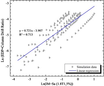
The results of analytical fragility curves based on the results of incremental dynamic (IDA) analysis are very sensitive to the selection of the intensity measures. Therefore, in the first step, there are different eleven intensity measures are considered to check the criteria of efficiency, practically and proficiency of them. Consideration of the efficiency, practically are in log-normal space. Figs. 4 to 14 are the results of linear regression analysis on the log-normal space in longitudinal directions. The spectral intensity measures are from Sa (0.2T1,5 %) till Sa (2T1,5 %) with the increment of 0.2 are considered. The effects of period of the bridge ( 0.51 s) on the sensitivity of the intensity measure are tabulated in Table 3.
Parameters and are the linear regression analysis. The efficiency of the intensity measure is studied with the parameters . The parameter is the practicality of the intensity measure. The composite measure of the practicality and the efficiency are in parameter . The lower values of show the more proficient intensity measure. From the results, it has been indicated that the Sa (1.2T1,5 %) is the proficient intensity measure which improves the results comparing to PGA more that 13 %.
Table 3Comparisons of regression values of PGA and spectral intensity measures and dispersion values
IM | Difference | ||||
PGA (g) | 0.014 | 0.82 | 15.73674 | 19.1911463 | 13.26777 |
Sa (0.2T1,5 %) | 0.011 | 0.82 | 26.18176 | 31.9289756 | 88.44751 |
Sa (0.4T1,5 %) | 0.009 | 0.66 | 15.74064 | 23.8494545 | 40.76149 |
Sa (0.6T1,5 %) | 0.010 | 0.88 | 37.9044 | 43.0731818 | 154.2216 |
Sa (0.8T1,5 %) | 0.012 | 0.9 | 16.75135 | 18.6126111 | 9.853202 |
Sa (T1,5 %) | 0.014 | 0.91 | 16.29959 | 17.9116374 | 5.715996 |
Sa (1.2 T1,5 %) | 0.016 | 0.9 | 15.24885 | 16.9431667 | 0 |
Sa (1.4T1,5 %) | 0.018 | 0.9 | 33.67418 | 37.4157556 | 120.8309 |
Sa (1.6T1,5 %) | 0.020 | 0.76 | 15.74987 | 20.7235132 | 22.31192 |
Sa (1.8T1,5 %) | 0.020 | 0.72 | 29.19925 | 40.5545139 | 139.3562 |
Sa (2T1,5 %) | 0.020 | 0.676 | 15.75478 | 23.3058876 | 37.55332 |
Fig. 4Simulated maximum column drift ratio (as EDP) of bridge as a function of PGA (as IM) of earthquake motions
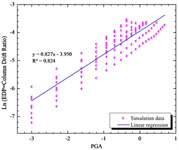
Fig. 5Simulated maximum column drift ratio (as EDP) of bridge as a function of Sa (0.2T1,5 %) (as IM) of earthquake motions
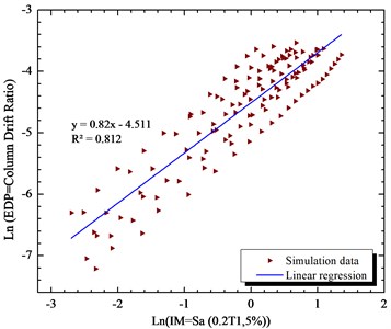
Fig. 6Simulated maximum column drift ratio (as EDP) of bridge as a function of Sa (0.4T1,5 %) (as IM) of earthquake motions
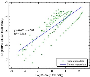
Fig. 7Simulated maximum column drift ratio (as EDP) of bridge as a function of Sa (0.6T1,5 %) (as IM) of earthquake motions
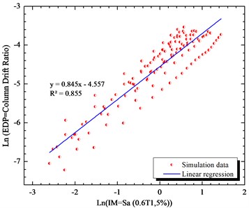
Fig. 8Simulated maximum column drift ratio (as EDP) of bridge as a function of Sa (0.8T1,5 %) (as IM) of earthquake motions
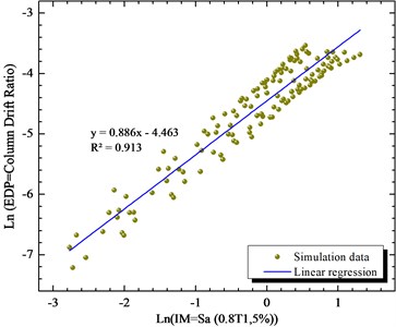
Fig. 9Simulated maximum column drift ratio (as EDP) of bridge as a function of Sa (T1,5 %) (as IM) of earthquake motions
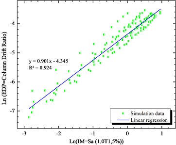
Fig. 10Simulated maximum column drift ratio (as EDP) of bridge as a function of Sa (1.2T1,5 %) (as IM) of earthquake motions
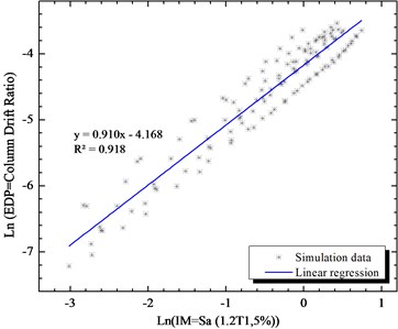
Fig. 11Simulated maximum column drift ratio (as EDP) of bridge as a function of Sa (1.4T1,5 %) (as IM) of earthquake motions
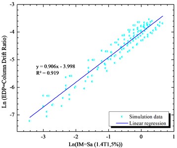
Fig. 12Simulated maximum column drift ratio (as EDP) of bridge as a function of Sa (1.6T1,5 %) (as IM) of earthquake motions
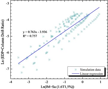
Fig. 13Simulated maximum column drift ratio (as EDP) of bridge as a function of Sa (1.8T1,5 %) (as IM) of earthquake motions
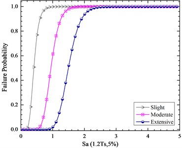
Therefore, we have developed the fragility curve of the bridge for this intensity measure as its shown in Figs. 15 to 16 for PGA and Sa (1.2T1,5 %). Obviously, the failure probability presented with the Sa (1.2T1,5 %) intensity measure is more accurate than PGA because the difference in their proficiency which is about 13 %.
Fig. 14Simulated maximum column drift ratio (as EDP) of bridge as a function of Sa (2T1,5 %) (as IM) of earthquake motions
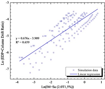
Fig. 15Fragility curves of the bridge pier respect to PGA
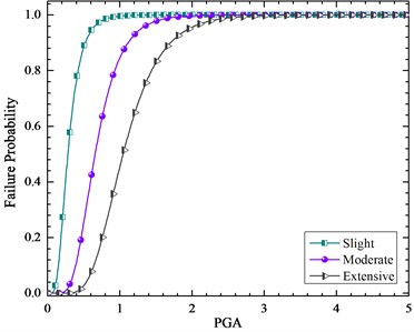
Fig. 16Fragility curves of the bridge pier respect to Sa (1.2T1,5 %)
7. Conclusions
In this paper, a detailed highly skewed highway bridge was studied. An attempt was made to try to develop the analytical fragility curve accurately. The first step in developing the analytical fragility curve is to choose an optimal intensity measure which is the most proficient one. Therefore, a sensitive analysis has been done on the proficiency of the intensity measures (1.2T1, 5 %) is the proficient intensity measure of the 60 skewed bridge in this study. The analytical fragility curves have been drawn for the considered intensity measure which prepares more accurate failure probability of the bridge for different performance levels.
References
-
Cornell C. A., Krawinkler H. Progress and challenges in seismic performance assessment. PEER Center News, Vol. 3, Issue 2, 2000, p. 1-3.
-
Kaynia A. M. Guidelines for Deriving Seismic Fragility Functions of Elements at Risk: Buildings, Lifelines, Transportation Networks and Critical Facilities. SYNER-G Reference Report 4, Publications Office of the European Union, Luxembourg, 2013.
-
Deierlein G., Krawinkler H., Cornell C. A framework for performance-based earthquake engineering. Pacific Conference on Earthquake Engineering, Vancouver, B.C., Canada, 2004.
-
Shinozuka M. Development of bridge fragility curves based on damage data. An International Journal of Earthquake Engineering and Engineer Seismology, Vol. 2, Issue 2, 2000, p. 35-45.
-
Yamazaki F., Hamada T., Motoyama H., Yamauchi H. Earthquake damage assessment of expressway bridges in Japan. Technical Council on Lifeline Earthquake Engineering Monograph, Vol. 16, 1999, p. 361-370.
-
Karim K. R., Yamazaki F. Comparison of empirical and analytical fragility curves for RC bridge piers in Japan. 8th ASCE Specialty Conference on Probabilistic Mechanics and Structural Reliability, 2000.
-
Hwang H., Liu J., Chiu Y. Seismic Fragility Analysis of Highway Bridges. Technical Report, Center for Earthquake Research and Information, University of Memphis, Memphis, 2001.
-
Choi E., DesRoches R., Nielson B. Seismic fragility of typical bridges in moderate seismic zones. Engineering Structures, Vol. 26, Issue 2, 2004, p. 187-199.
-
Bayat M., Daneshjoo F., Nisticò N. Probabilistic sensitivity analysis of multi-span highway bridges. Steel and Composite Structures, Vol. 19, Issue 1, 2015, p. 237-262.
-
Bayat M., Daneshjoo F., Nisticò N. A novel proficient and sufficient intensity measure for probabilistic analysis of skewed highway bridges. Structural Engineering and Mechanics, Vol. 55, Issue 6, 2015, p. 1177-1202.
-
Bayat M., Daneshjoo F., Nisticò N. The effect of different intensity measures and earthquake directions on the seismic assessment of skewed highway bridges. Earthquake Engineering and Engineering Vibration, Vol. 16, Issue 1, 2017, p. 165-179.
-
Bayat M., Daneshjoo F. Seismic performance of skewed highway bridges using analytical fragility function methodology. Computers and Concrete, Vol. 16, Issue 5, 2015, p. 723-740.
-
Pan Y., Agrawal A. K., Ghosn M., Alampalli S. Seismic fragility of multi-span simply supported steel highway bridges in New York State. II: Fragility analysis, fragility curves, and fragility surfaces. Journal of Bridge Engineering, Vol. 15, Issue 5, 2010, p. 462-472.
-
Nielson G. B. Analytical Fragility Curves for Highway Bridges in Moderate Seismic Zones. Georgia Institute of Technology, In Partial Requirement for the Requirement for Doctor of Philosophy, 2005.
-
Mander J. B. Seismic Design of Bridge Piers. Research Report 84-2, Department of Civil Engineering, University of Canterbury, Christchurch, New Zealand, 1984.
-
Quantification of Building Seismic Performance Factors. FEMA P695, Washington, DC, 2009.
-
Cornell A. C., Jalayer F., Hamburger R. O. Probabilistic basis for 2000 SAC federal emergency management agency steel moment frame guidelines. Journal of Structural Engineering, Vol. 128, Issue 4, 2002, p. 526-532.
-
Padgett Jamie E., Nielson Bryant G., Des Roches R. Selection of optimal intensity measures in probabilistic seismic demand models of highway bridge portfolios. Earthquake Engineering and Structural Dynamics, Vol. 37, Issue 5, 2008, p. 711-725.
-
Multi-hazard Loss Estimation Methodology. Earthquake Model. HAZUS99 User’s Manual. Federal Emergency Management Agency, Washington, DC, 1999.
-
Choi E., DesRoches R., Nielson B. Seismic fragility of typical bridges in moderate seismic zones. Engineering Structures, Vol. 26, Issue 2, 2004, p. 187-199.
-
Yi J.-H., Kim S.-H., Kushiyama S. PDF interpolation technique for seismic fragility analysis of bridges. Engineering Structures, Vol. 29, Issue 7, 2007, p. 1312-1322.
Cited by
About this article

