Abstract
The purpose of this study is to investigate the characteristics of vibration isolation system with a single degree-of-freedom (SDOF) and a two-degree-of-freedom (2DOF) respectively based on the high-static-low-dynamic-stiffness (HSLDS). This model consists of a simple configuration connecting a vertical spring and a pair of oblique springs. The restoring force of the isolation system is approximated to linear and cubic stiffness by applying the Maclaurin series expansion. The dynamic equations of the SDOF and 2DOF are established for the harmonic force excitation. The frequency-amplitude response equation of the SDOF is obtained by employing the harmonic balance method (HBM) and is demonstrated in the classical Runge-Kutta method. The solution stability is ensured by applying the Floquet theory. Effects on the frequency response curves (FRCs) for the damping ratio and excitation amplitude are explored and discussed. The force transmissibility (FT) is defined to evaluate the vibration suppression capability. Effects on the FT of the SDOF and 2DOF for the excitation amplitude, mass ratio, and damping ratio are investigated. An experimental investigation of the SDOF is carried out to evaluate the actual attenuation performance in comparison with the equivalent linear system (ELS). The simulation and experimental results show that the HSLDS system with harmonic force excitation demonstrates hardening stiffness with multi-valued solutions. The occurrence of jump phenomenon is observed and explained by the stiffness variation. The system response and resonance frequency are affected by the excitation amplitude and damping ratio. The HSLDS system outperforms the ELS in a low frequency range if an appropriate mass is mounted. It is excited by a proper force and owns a suitable damper, which offers a theoretical guidance for the design and application of a novel HSLDS isolator.
1. Introduction
Undesirable vibration is a harmful effect that affects practical equipment, high-precision machinery and human health. It is evident that the bandwidth of vibration isolation is often limited by the mounted stiffness element required to support a static load. To overcome this limitation, the High-static-low-dynamic-stiffness (HSLDS) mechanism was put forward, what results in low a natural frequency with a small static displacement. Whilst it maintains locally low stiffness near equilibrium and static load bearing, which reduces the natural frequency and extends the frequency isolation region [1]. When there is an isolator, whose dynamic linear stiffness is zero or near zero, it is called as a quasi-zero-stiffness (QZS) isolator [2]. The isolation system with HSLDS characteristic has been well established both theoretically and experimentally in recent literatures, and has recently been the subject of growing interest of both engineers and researchers. There are many approaches to get the HSLDS characteristics. Carrella and Wu investigated vibration isolators with the HSLDS property via a combination of a mechanical spring and magnets [3, 4]. Zhou proposed a QZS isolator with a cam-roller mechanism [5]. Li presented a device using a magnetic spring combined with rubber membranes to suppress vibration [6]. Meng concerned the quasi-zero-stiffness by combining in parallel a negative disk spring with a linear positive spring [7]. Liu developed a quasi-zero-stiffness by connecting the Euler buckled beam mechanism and a linear spring [8]. Zhou used a pair of electromagnets and a permanent magnet to build a tunable semi-active isolator with the HSLDS property [9]. Yashikazu applied super elastic Cu-Al-Mn shape memory alloy bars to develop a QZS isolator [10].
The above mentioned literatures as well as other literatures concerning HSLDS isolators have been more focused on the mechanism and theoretical analysis of a single-degree-of-freedom (SDOF)-HSLDS system. Experimental investigations and theoretical analysis of the SDOF-HSLDS system have been seldom reported, and their practical applications are even rare. Little changes were made in the control strategy to expand the isolation range to a lower frequency but with a high isolation performance. Unlike previous studies, the aim of this paper is to develop a SDOF-HSLDS and two-degree-of-freedom (2DOF)-HSLDS system experimentally and theoretically that can be useful for the elimination of line spectra of noise radiated from a submarine.
In this paper, an investigation of a SDOF isolation system and 2DOF isolation system with the HSLDS characteristics was presented. The harmonic balance method (HBM) was applied to achieve the amplitude frequency characteristic equation, and the stable and unstable solutions were derived based on the Floquet theory. The effects of the excitation amplitude, mass ratio and damping ratio on frequency response curves (FRCs) and force transmissibility (FT) of the HSLDS vibration isolation system were investigated analytically and experimentally as compared with that of the equivalent linear system (ELS).
2. Vibration isolation of SDOF system
2.1. Description of general model
The system depicted in Fig. 1 is a parallel connection of two oblique linear springs with identical stiffness and a vertical linear spring with identical stiffness . The oblique springs are hinged at and , and connected with the vertical spring at point . The configuration geometry is decided by horizontal distance from point to and initial height , while denotes the vertical displacement from the initial unloaded position caused by the force .
Fig. 1Schematic representation of isolator based on HSLDS
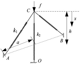
a)
b)
The general equation between the force and the displacement can be derived as:
Noting that, Eq. (1) can be remade in the dimensionless form as:
where , , , . Approximating Eq. (2) to the third order by using the Maclaurin series expansion, one yields:
The dimensionless dynamic stiffness can be obtained by differentiating Eq. (3) to :
The dimensional form of Eq. (4) is . It is clear that the oblique springs can reduce the positive stiffness so that the linear natural frequency is smaller in the isolation range; and they introduce the cubic stiffness term so that the peak response bends to higher frequencies, what potentially reduces the frequency region.
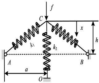
The SDOF system is depicted in Fig. 2. It includes a rigid mass suspended on a three-springs mount in parallel with a viscous damperexcited by harmonic excitation . The mass moves in the vertical direction through the guide rod and bushing. By applying the Newton’s second law, the motion equation of SDOF system can be expressed as.
where and The following dimensionless variables are introduced as , , , , . Eq. (5) can be expressed in the dimensionless form as:
What is a hardening Helmholtz-Duffing oscillator and primes.
Fig. 2Structural model of SDOF system with HSLDS characteristic: 1 – loading platform, 2 – oblique spring, 3 – guide device, 4 – pillar, 5 – vertical spring, 6 – base plate, 7 – linear bearing, 8 – sliding rod
a)
b)
2.2. Amplitude-frequency equation and stability analysis
Considering that the vibration isolation system with the HSLDS characteristic is a strongly nonlinear, the Mathieu equation criterion and perturbation methods are invalid. The corresponding steady-state approximate solution is obtained by using the general Hill equation and HBM [11].
Applying the HBM, the solution of Eq. 6, denoted by , is supposed as a truncated Fourier series plus a small perturbation. The system response is given by:
where , and are Fourier parameters of harmonic balance solution and is the truncated order. In particular, substituting Eq. (7) into Eq. (6) with 3, Eq. (6) can be transferred as:
where the functional dependence of , , , , and on the parameters , , is shown in Appendix. Since the substitution introduced seven parameters into the system, which can be obtained by the coefficients and of harmonic and equated to zero respectively ( 1,…, 3, 1,…, 9, 1,…, 9). The linearized variational equation of the Eq. (8) can be written as:
It is worthy of noting that the stability analysis of Eq. (7) is changed to the general Hill equation. According to the Floquet theory [12], the solution of Eq. (10) can be assumed to be:
where is the characteristic Floquet exponent. Eq. (10) is substituted into Eq. (9), and the coefficients of the same harmonics are equated and ignore the higher harmonics. This leads to an infinite set of linear homogeneous equations 0, where is the column vectors , is the matrix of coefficients. Following the procedure stated in Ref. [12], 0 exists an nontrivial solutions if the determinant of , denoted by , vanishes. Thus, the stable (respectively, unstable) condition is determined by whether is positive (negative), the boundary between the stable and unstable regions is 0.
This paper aims to find the primary resonance response. The corresponding steady-state harmonic solution is supposed to be , which leads to the following amplitude-frequency relation according to the Appendix:
With the term containing eliminated, Eq. (11) can be expanded and arranged. The amplitude-frequency equation can be yielded as:
With the term containing eliminated, Eq. (11) can be expanded and arranged. The phase-frequency equation can be yielded as:
The two positive solutions for , which are the resonant and non-resonant branches in the frequency response function, can be solved analytically in Eq. (12):
The peak response can be reached when and are equal. Thus, the peak response of and corresponding are found as follows:
Noting that 1 and according to the procedure shown in Appendix, Eq. (9) can be written as:
where , , .
According to the Floquet theory, the solution of Eq. (16) can be assumed to be:
By substituting Eq. (17) into Eq. (16) and applying the HBM, one can conclude that:
With the term containing and neglected, the coefficients of harmonics and are equated to zero respectively, what can be derived as:
Nontrivial solutions exist only when the determinant of the matrix in Eq. (19), denoted by , vanishes, waht can be derived as:
Eq. (20) is the boundary between the stable and unstable regions and the unstable regions can be determined by .
2.3. Effects on FRCs for damping ratio and excitation amplitude
In this section, the effects of the damping ratio and excitation amplitude on the shape of the FRCs are investigated by the controlling variables method. It is worthy of noting that the steady-state solution is obtained only by considering the component of the primary resonance response, where the classical Runge Kutta method needs to be used to validate the accuracy of the appropriate solutions obtained by HBM. These curves are plotted in Figs. 3-5 for three distinguishable cases, where the red solid line and the blue dotted line of the FRCs represent the stable and unstable solutions, respectively, and the symbols black “o” and green “*” denote the numerical solution and peak response, respectively. It can be observed from the Figs. 3-5, the analytical and numerical results fit in well.
Fig. 3FRCs of system with different damping ratios where f= 0.5 and ξ= 0.1, 0.2, 0.3
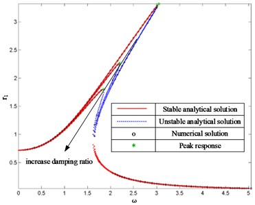
Fig. 4FRCs of system with different excitation amplitudes where ξ= 0.1 and f= 0.5, 1, 1.5
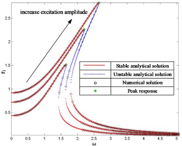
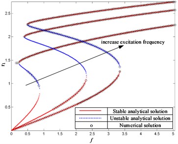
Fig. 5Dependence of response amplitude on excitation amplitude where ξ= 0.1 and ω= 1.6, 2, 2.2
As shown in Fig. 3, an increase in the damping ratio results in a decrease in the resonance frequency and peak response when the excitation amplitude is fixed. The unstable regions also decreases as the damping radio increases and the FRCs approach is equal at lower or high frequencies. The FRCs of the harmonic response are bent to the right, as they are intended for the hardening stiffness characteristic. However, the FRCs will tend to the linear form when the damping ratio is excessive.
In the above analysis, the excitation amplitude of the HSLDS system is always fixed. It is interesting to study the effects of excitation amplitude on the FRCs when the damping ratio is fixed. The FRCs with different excitation amplitudes are plotted in Fig. 4. It can be seen obviously that larger excitation amplitude can result in both larger resonance frequency and peak response. An increase in the excitation amplitude yields an increase in the unstable region. The FRCs changes are larger with larger excitation amplitude at lower frequencies while that approaches are the same at high frequencies.
The dependence of the response amplitude on the excitation amplitude is plotted in Fig. 5. By observing Fig. 5, sometimes the number of steady-state solution is only one, sometimes it is three, depending on the initial conditions. The region of existing three stable solutions extends as the excitation frequency increases.
2.4. FT definition
The FT is defined as the ratio between the amplitude of force transmitted to the base and amplitude of the excitation force [13]:
The contains the elastic force and damping force, which can be expressed by:
Thus, substituting Eq. (12) and Eq. (13) into Eq. (22) and only considering the dynamic force, the FT of the HSLDS isolator can be expressed by:
The peak FT corresponds to the peak response . Substituting Eq. (15) into Eq. (23), one yields:
where . For the ELS, the mathematical expression of FT is given in dimensionless quantities by:
2.5. Effects on FT for damping ratio and excitation amplitude
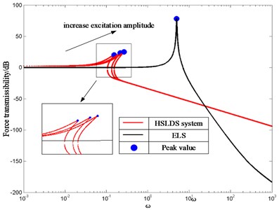
The Effects on the FT of the HSLDS system and the ELS for the damping ratio and excitation value are plotted in Figs. 6-7, where the red solid parts and black solid parts represent the FT of the HSLDS system and the ELS respectively, the symbols “●” denote the peak amplitude of FT, and the FT values are expressed in dB, i.e. as 20 . By inspecting Fig. 6-7, one conclusion can be obtained that the isolation performance of the HSLDS system will be better or worse than that of the ELS depending on the excitation frequency and system parameters.
As shown in Fig. 6, larger damping ratio yields both smaller peak amplitude and smaller resonance frequency of the FT when the excitation amplitude is fixed. However, the excessive damping ratio is detrimental to the isolation performance of HSLDS system at high frequencies. As for the ELS, larger damping ratio yields smaller peak amplitude, while the resonance frequency remains unchanged. As compared with the ELS, the HSLDS system has a smaller initial frequency, wider isolation band and better isolation performance. But when the excitation frequency is excessive, the FT of the HSLDS system is greater than that of the ELS.
As shown in Fig. 7, an increase of the excitation amplitude yields both larger peak value and larger resonance frequency of the FT when the damping ratio is fixed. The FTs of the different excitation amplitudes approach to the same level at higher frequencies. As for the ELS, the peak amplitude and resonance frequency are independent from the excitation amplitude. As compared with the ELS, the HSLDS system has a smaller initial frequency, wider isolation band and better isolation performance; but the excessive excitation frequency will deteriorate the isolation performance of the HSLDS system.
Fig. 6FT of HSLDS system and its ELS with different damping ratios where f= 0.5 and adjusted ξ= 0.1, 0.2, 0.3
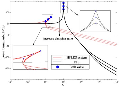
Fig. 7FT of HSLDS system and its ELS with different excitation amplitudes where ξ= 0.1 and f=0.5,1,1.5 0.5, 1, 1.5
2.6. Experimental investigation
To assess the attenuation performance of the proposed SDOF-HSLDS system and to validate the nonlinear phenomenon presented in the previous section, a prototype experiment is carried out. The experimental apparatus of the HSLDS is shown in Fig. 8. The mass is supported by the vertical spring and moves in the vertical direction through the guide rod and bushing. The HSLDS isolator was installed at a rubber vibration isolation system. A vibration exciter powered by a power amplifier is mounted on top of the mass to provide external force in the vertical direction. Between the exciter and the mass, a force sensor is installed to measure the excitation force. Another force sensor is placed underneath the base plate of the HSLDS device to measure the transmitted force during vibration. A data acquisition analyzer is used to extract the output signal from the sensors. A personal computer is used to handle the I/O data operation for the whole measuring system. The experimental setup can be divided into three steps: excitation system, data acquisition system and measured subject. The isolator parameters are shown in Table 1.
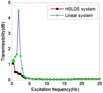
The vibration isolation performance is assessed by the FT, which is defined as the ratio of the root mean square (RMS) value of the force transmitted to the base, and as of the RMS value of the excitation force. A linear system is used for a benchmark comparison. The external excitation frequency is varied from 0.5 to 25 Hz. In the actual experiments, two series of experiments are conducted for two series of excitation conditions. The excitation force keeps constant at the level of 20 N for the Case I and keeps constant at the level of 10 N for the Case II. Fig. 9 shows the transmissibility of different levels of excitation force. It is evident that the linear system has the resonance peak of about 2.1 Hz, while the HSLDS system is not involved in the resonance.
Table 1Physical parameters for making experimental apparatus
Parameter | Original value |
0.4 (N/mm) | |
0.711 (N/mm) | |
2.3 (kg) | |
70 (mm) | |
90 (mm) | |
56.5 (mm) |
Fig. 8Experimental setup of HSLDS isolator
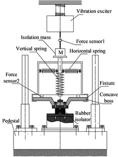
a) Schematic representation of isolator
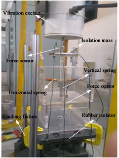
b) Prototype of experimental apparatus
Fig. 9Experimental comparison of force transmissibility between HSLDS and ELS at different levels of excitation force
a) Case I
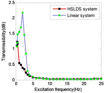
b) Case II
Theoretically, the HSLDS system has a bended resonance peak, but a small damping can make the peak vanish. It is because that the stiffness of the HSLDS system about the equilibrium is close to zero so that the resonance peak has shifted to a lower frequency. The HSLDS system starts the effective attenuation from 0.3 Hz where the transmissibility value is less than one, while the ELS can only start from 3 Hz. The performance of the HSLDS system appears to be equivalent to that of ELS in the high-frequency band after 4 Hz. It can be seen obviously that the performance of the proposed HSLDS system is superior to the ELS in terms of the isolation frequency region, which validates the concept of HSLDS isolator usage to lower the dynamic stiffness to a positive stiffness.
3. Vibration isolation of 2DOF system
3.1. 2DOF nonlinear isolation system and equivalent linear isolation system
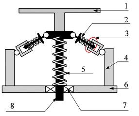
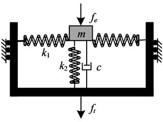
In this section the 2DOF nonlinear (hereinafter referred to as “N-N”) isolation system shown in Fig. 8 is investigated to see if this isolation performance is superior to the corresponding 2DOF linear (hereinafter referred to as “L-L”) isolation system. The N-N isolation system, which includes the mass of vibration object , together with a vertical stiffness , a viscous damper and two horizontal stiffness ; and the mass of the intermediate object , in parallel with a vertical stiffness , a viscous damper and two horizontal stiffness , consists of two SDOF isolators shown in Fig. 10(a). is the force transmitted to the base, and is the excitation force. and denote the vertical displacement of and , respectively.
Fig. 10Schematic of N-N and L-L isolator
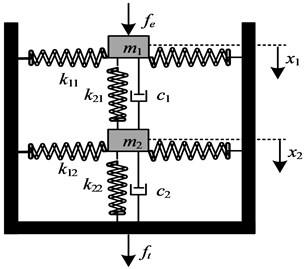
a) N-N configuration
b) L-L configuration
In the analysis above, the motion equation of the SDOF system with the HSLDS characteristic in Fig. 2 can be approximated by:
Thus, the motion equation of the N-N isolation system under harmonic force excitation can be expressed as:
Eq. (27) can be transferred into the matrix form as:
where:
By introducing the dimensionless parameters as follows:
Eq. (28) can get the dimensionless dynamic equation:
where:
By applying the HBM [14-15], set the Eq. (29) solution as:
where , and represent the Fourier coefficient of harmonic balance solution and truncated order, respectively. The first and second derivatives of Eq. (30) are given by:
By substituting Eq. (31) into Eq. (29), one can obtain the appearance of high-order term. According to the orthogonally of trigonometric functions [16-17], one can reach:
where:
Supposing that 1, the solution of Eq. (29) can be assumed as:
By substituting Eq. (34) into Eq. (29) and setting the coefficients of the terms including and to be zero respectively and ignoring the higher harmonics, one yields the implicit amplitude-frequency equation in the form of matrix derived as:
where:
The dimensionless force transmitted to the base is:
where , , .
Assuming that , the force magnitude can be obtained as:
where .
According to the Eq. (21), the FT of the N-N isolator can be expressed by .
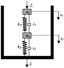
For a comparison, two pairs of horizontal springs are removed, and the corresponding linear isolator is shown in Fig. 10(b). The dimensionless dynamic equation for the L-L isolation system can be expressed as:
where:
The dimensionless force transmitted to the base is:
where:
Assuming that , the force magnitude can be obtained as:
where .
According to the Eq. (21), the FT of the L-L isolator can be expressed by .
3.2. Effect of parameters on FT
In the above analysis, the FT is closely related to the excitation amplitude, mass ratio and damping ratio. It is interesting to study the effects of different system parameters on the FT with the help of the controlling variable method. The FTs of N-N and L-L isolation system are plotted together to compare the isolation performance, expressed in dB. A given set of parameters –0.02, 4.47, 0.98, 4.47, 1 are chosen to conduct the following investigation.
Fig. 11 shows the FT of N-N isolator and L-L isolator with the changed excitation amplitude. It can be seen that the first and second resonance frequencies and corresponding peak of FTs increase obviously as the excitation amplitude increases. However, the FT of L-L isolator is not affected by the excitation amplitude. The FT of the N-N isolator is larger than that of the L-L isolator at low frequencies while the FT of the N-N isolator changes to a smaller value than that of the L-L isolator at frequencies greater than the first resonance frequency. Thus, one can conclude that the N-N isolator outperforms than that of the L-L isolator at high frequencies.
Fig. 11FT of N-N isolator and L-L isolator with different excitation amplitudes where ξ1=ξ2= 0.03, μ= 2 and f= 0.01, 0.1, 0.5
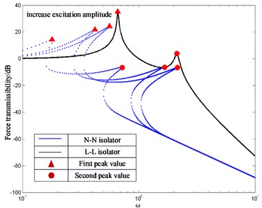
Fig. 12 shows the effect on the FT with the changed mass ratio. For the N-N isolator, it can be seen that an increase of the mass ratio will result in an increase of the first resonance frequency and corresponding peak of FTs, but in a decrease of the second resonance frequency and corresponding peak of FTs. However, for the L-L isolator, one can conclude that the first resonance frequency, corresponding FT peak and the second resonance frequency decrease, while the second peak of FTs increases as the mass ratio increases. Thus, an increase of the mass ratio can broaden the frequency region of isolation, but a decrease of the isolation performance can occur near the second resonance frequency.
In the previous sections, the isolation performance of the N-N isolator is better than the L-L isolator for specific values of damping ratio. Here the effects of the damping ratio on the FT are investigated in Fig. 11 when the excitation amplitude and mass ratio are fixed. Fig.13(a) illustrates that the damping ratio in the lower stage is fixed and the damping ratio of the upper stage is varied. By inspecting Fig. 13(a), one can conclude that the first resonance frequency and corresponding peak of the N-N isolator and L-L isolator are hardly changed after the damping ratioincreased. But the second resonance frequency, corresponding peak of the N-N isolator and second peak of the L-L isolator reduce with the increase of the damping ratio , while the second resonance frequency of the L-L isolator remains unchanged. But an increase of the damping ratio will deteriorate the isolation performance at frequencies greater than the second resonance frequency. Fig. 13(b) illustrates that the damping ratio in the upper stage is fixed, the damping ratio of the lower stage is varied. By inspecting Fig. 13(a), one can conclude that the first resonance frequency, corresponding peak and second resonance frequency of the N-N isolator decrease as the damping ratio increases, while the second peak increases. The first resonance frequency and corresponding peak of the L-L isolator decrease as the damping ratio increases, while the second resonance frequency and corresponding peak remain unchanged. Thus, it is preferable to have properly high damping ratio to control the response at the second resonance frequency and as a small damping ratio to reduce the transmitted force.
Fig. 12FT of N-N isolator and L-L isolator with different mass ratios where ξ1=ξ2= 0.03, f= 0.1 and μ= 1, 2, 3
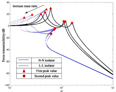
Fig. 13FT of N-N isolator and L-L isolator with different damping ratios
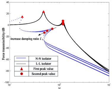
a) Effect of regular and variable where 0.1, 0.03, 2 and 0.01, 0.03, 0.05
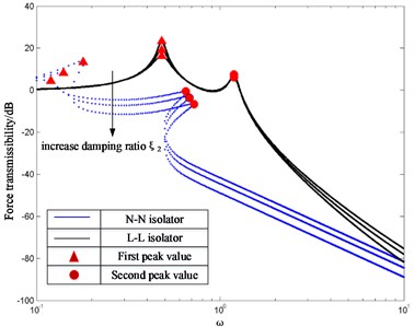
b) Effect of regular and variable where 0.1, 0.03, 2 and 0.01, 0.03, 0.05
4. Conclusions
In this study, the characteristics of the vibration isolation system based on the HSLDS have been investigated theoretically and experimentally. The isolation system consists of a vertical spring providing a positive stiffness and of two auxiliary springs providing a negative stiffness. HSLDS isolation system is termed as follows: SDOF and 2DOF. The effects of excitation amplitude, mass ratio, and damping ratio on FRCs and FTs are analyzed. The conclusions can be summarized as follows:
Firstly, for the SDOF, the effects of the excitation amplitude decrease and the damping ratio increase are properly beneficial to the isolation performance as compared with the ELS, but they degrade the performance at a higher frequency. The experimental results demonstrate that the HSLDS isolator is not involved into the resonance phenomena as compared with the ELS.
Secondly, for the 2DOF, if the excitation amplitude and damping ratio as well as the mass ratio and damping ratio decrease properly, the N-N isolator possesses smaller initial isolation frequency, wider isolation band and better isolation performance ad compared with the L-L isolator. The appropriate damper increase is also a feasible way to avoid the occurrence of jump phenomenon of the N-N isolator and to make this kind of HSLDS isolator performance better.
Thirdly, the introduction of the negative stiffness mechanism is an effective way to lower the resonance frequency, and the HSLDS isolation system can reduce the dynamic stiffness and hence can increase the frequency range of isolation.
Finally, the present study will provide a useful insight into the design principles when putting such a kind of low-frequency HLSDS isolator into practice. Future studies will extend the proposed design to the cases where loading excitations are more realistic and will evaluate the system performance in practical applications.
References
-
Shaw A. D., Neild S. A., Friswell M. I. Relieving the effect of static load errors in nonlinear vibration isolation mounts through stiffness asymmetries. Journal of Sound and Vibration, Vol. 339, 2015, p. 84-98.
-
Lan Chao Chieh, Yang Sheng An, Wu Yi Syuan Design and experiment of a compact quasi-zero-stiffness isolator capable for a wide range of loads. Journal of Sound and Vibration, Vol. 333, 2014, p. 4943-4858.
-
Carrella A., Brennan M. J., Waters T. P. On the design of a high-static-high-dynamic stiffness isolator using linear mechanical springs and magnets. Journal of Sound and Vibration, Vol. 315, 2008, p. 712-720.
-
Wu Wenjiang, Chen Xuedong, Shan Yuhu Analysis and experiment of a vibration isolator using a novel magnetic spring with negative stiffness. International Journal of Mechanical Sciences, Vol. 81, 2014, p. 207-214.
-
Zhou Jia Xi, Wang Xin Long, Xu Dao Lin, et al. Experiment study on vibration isolation characteristics of the quasi-zero-stiffness isolator with cam-roller mechanism. Journal of Vibration Engineering, Vol. 28, Issue 3, 2015, p. 449-455.
-
Li Qiang, Zhu Yu, Xu Dengfeng, et al. Negative stiffness vibration isolator using magnetic spring combined with rubber membrance. Journal of Mechanical Science and Technology, Vol. 27, Issue 3, 2013, p. 813-824.
-
Meng Lingshuai, Sun Jinggong, Wu Wenjuan Theoretical design and characteristics analysis of a quasi-zero stiffness isolator using a disk spring as negative stiffness element. Shock and Vibration, 2015, https://doi.org/10.1155/2015/813763.
-
Liu Xingtian, Huang Xiuchang, Hua Hongxing On the characteristics of quasi-zero stiffness isolator using Euler buckled beam as negative stiffness corrector. Journal of Sound and Vibration, Vol. 332, 2013, p. 3359-3376.
-
Zhou N., Liu K. Tunable high-static-low-dynamic stiffness vibration isolator. Journal of Sound and Vibration, Vol. 329, 2010, p. 1254-1273.
-
Araki Yoshikazu, Kimura Kosuke, Asai Takehiko, et al. Integrated Mechanical and material design of qua-zero-stiffness vibration isolator with superelastic Cu-Al-Mn shape memory alloy bars. Journal of Sound and Vibration, Vol. 358, 2015, p. 74-83.
-
Niu Fu, Meng Lingshuai, Juan Wen, et al. Design and analysis of a quasi-zero-stiffness isolator using a slotted conical disk spring as negative stiffness structure. Journal of Vibroengineering, Vol. 16, Issue 4, 2014, p. 1875-1891.
-
Ameer Hassan. On the local stability analysis of the approximate harmonic balance solutions. Nonlinear Dynamics, Vol. 4, 1996, p. 105-133.
-
Carrella A., Brennan M. J., Waters T. P., et al. Force and displacement transmissibility of a nonlinear isolator with high-static-low-dynamic-stiffness. International Journal of Mechanical Sciences, Vol. 55, 2012, p. 22-29.
-
Lu Zeqi, Brennan Michael J., Yang Tiejun, et al. An investigation of a two-stage nonlinear vibration isolation system. Journal of Sound and Vibration, Vol. 332, 2013, p. 1456-1464.
-
Gatti Gianluca, Kovacic Ivana, Brennan Michael J. On the response of a harmonically excited two degree-of-freedom system consisting of a linear and a nonlinear quasi-zero stiffness oscillator. Journal of Sound and Vibration, Vol. 329, 2010, p. 1823-1835.
-
Guo P. F., Lang Z. Q., Peng Z. K. Analysis and design of the force and displacement transmissibility of nonlinear viscous damper based vibration isolation systems. Nonlinear Dynamics, Vol. 67, 2012, p. 2671-2687.
-
Yang J., Xiong Y. P., Xing J. T. Dynamic and power flow behavior of a nonlinear vibration isolation system with a negative stiffness mechanism. Journal of Sound and Vibration, Vol. 332, 2013, p. 167-183.
Cited by
About this article

The research leading to these results has received funding from the National Natural Science Foundation of China (NSFC) under the Grants No. 51579242, No. 51509253 and No. 51679245. All the supports mentioned above are gratefully acknowledged.
