Abstract
This paper presents a novel approach for improving the estimation accuracy of the road profile for a vehicle suspension system. To meet the requirements of road profile estimation for road management and reproduction of system excitation, previous studies can be divided into data-driven and model based approaches. These studies mainly focused on road profile estimation while seldom considering the uncertainty of parameters. However, uncertainty is unavoidable for various aspects of suspension system, e.g., varying sprung mass, damper and tire nonlinear performance. In this study, to improve the estimation accuracy for a varying sprung mass, a novel algorithm was derived based on the Minimum Model Error (MME) criterion and a Kalman Filter (KF). Since the MME criterion method utilizes the minimum value principle to solve the model error based on a model error function, the MME criterion can effectively deal with the estimation error. Then, the proposed algorithm was applied to a 2 degree-of-freedom (DOF) suspension system model under ISO Level-B, ISO Level-C and ISO Level-D road excitations. Simulation results and experimental data obtained using a quarter-vehicle test rig revealed that the proposed approach achieves higher road estimation accuracy compared to traditional KF methods.
1. Introduction
Road profile is the main input of a vehicle suspension system and its characteristics have a significant effect on vehicle performance, especially on the aspects of ride comfort, road handling, and road profile measurements, which have been performed to evaluate the ride quality of newly constructed pavement, to monitor the condition of road networks in road management systems, and to investigate the influence of fatigue, fuel consumption, and tire wear [1, 2]. Poor road conditions will raise the operating costs of goods transportation, and moreover, an increase in the dynamic axle loads will adversely affect the durability of roads [1, 2]. Therefore, the detection and estimation of road conditions has become a topic of particular interest for road information management, as well as vehicle dynamic control, and has increasing attracted attention [2, 3]. An accurate knowledge of the road profile is crucial for a better understanding of vehicle suspension system design [4].
Currently applied road estimation methods can be roughly divided into three categories [5], i.e. direct measurement [5, 6], non-contact measurement [7, 8] and system response-based estimation [9, 10]. Among these, due to lower costs and reduced measurement contamination (e.g. using laser or other visual sensors), the system response-based estimation method is most frequently used for road excitation estimation, and it can be further divided into two categories, i.e. data-driven and model-based. The former approach usually requires comprehensive training data. To this end, vehicle dynamic responses has been utilized to estimate the road profile in the time domain based on a nonlinear suspension model and an Adaptive Neuro Fuzzy Inference System (ANFIS) algorithm, and the simulation results showed that ANFIS provides better estimation performance than other data-driven methods [11]. Knowing that a higher accuracy estimation of road excitation can be obtained using the ANFIS method, an artificial neural network (ANN) approach was designed to estimate the road profile [12]. This method incorporated a validated vehicle ADAMS model to analyze road profile data. A comparison of results from the estimated road by ANN and the target road generated by ADAMS showed that the proposed method is effective. However, this study did not take into account the effects of cornering. Further to this, a data processing algorithm was proposed to estimate road profiles from the dynamic responses measured on the vehicle and validated using experimental data obtained from simulations and real measurements [13]. The proposed method could be applied to extract valuable statistical information on road roughness. Accelerometers data has also been adopted to estimate the road profile, which was accurately classified through the axles and body accelerations [14]. On the other hand, a model-based approach can deal with unforeseen situations that are not included in the training data set of the data-driven approach. Road profiles have been generated using vehicle sensors to control the active suspension for improving vehicle performance [15]. Preview feedback control and signal filtering was adopted to control the actuators. The simulation and experimental results showed that the method has a positive effect on vehicle ride comfort. This method could also be used in unmanned vehicles. The jump-diffusion process-based state estimator was considered along with the observer for road profile estimation and the road was evaluated using experiments and simulations [16]. A cloud-based implementation was also developed to facilitate information access and fast computation. The aforementioned approach could be used in practice. Another suggested approach for estimating the road profile is the adaptive observer based Q-parameterization [17]. Experimental results on the rear-left corner of a 1:5 scale vehicle was used to study and validate the road profile estimation. Based on the results, accuracy of the proposed method was at least 70 %. The developed approach could be used as an online road profile. A sliding mode observer was utilized to estimate the road profile and compared with experimental results showing the robustness of the proposed method [18, 19]. In addition, the Kalman Filter (KF) plays an important role in the state estimation field [20]. A real-time estimation method was developed to estimate the road profile based on a KF and experimental results showed high accuracy [6]. Moreover, dynamic responses were used to estimate the road profiles based on KF in a stochastic framework and validated using experimental data obtained from simulations and real measurements [13].
Model accuracy is an important requirement of the model-based observer. However, in practice the suspension system model is a multi-dimensional system. The system parameters are uncertain, due to variations in sprung mass, damping and tire stiffness. Uncertain system parameters can cause degradation in the state estimation quality [21, 22]. To improve the estimation accuracy caused by varying system parameters, the Minimum Model Error (MME) approach is proposed [23]. Previously, the approach was successfully used to estimate satellite altitude [24, 25]. The MME criterion method uses an objective function to solve the MME by using the minimum value principle [26].
In this paper, a novel method for efficient road profile estimation based on a KF and MME algorithm is proposed by considering the sprung mass variation. This method can be described as follows. First, the states of the suspension system at the current step and next step are estimated using the KF approach. Second, the model error matrix is deduced by MME criterion algorithm using information obtained from the KF. Then, the joint MME criterion and KF approach is used to modify the suspension system model so that the state estimation of the road profile can be achieved at the new step. Finally, the estimated road profile information at the new step is used as the initial state for the following step. The algorithm was implemented as a simulation and experiments were performed with a quarter-vehicle. The results showed that the proposed method produces a more accurate road profile estimation than traditional KF.
This paper evaluates the ability of the novel algorithm to improve the state estimation accuracy of the suspension system. Their contributions presented in this paper are:
• A novel idea to adjust the varying sprung mass depending on the MME criterion for the modified suspension system model;
• A proposed method of road profile estimation combining the MME criterion with the KF algorithm;
• A quarter suspension test rig is adopted to validate the MME and KF (MME&KF). Results showed the proposed method achieves better road estimation accuracy.
To further improve the accuracy of road estimation for the suspension system, this paper introduces an approach to evaluate the road profile state precision within a suspension system. The paper is organized as follows. Section 2, a quarter model of a vehicle suspension is described. The joint state-parameter KF&MME criterion approach are derived in Section 3. Section 4 shows the test and simulation results of proposed method. Finally, the conclusions are summarized in Section 5.
2. Vehicle suspension model
2.1. Quarter vehicle suspension model
The quarter vehicle model, which is the most commonly used model for suspension systems, is presented in this section. Due to the nonlinearity of the practical quarter suspension, linearization of the quarter suspension model is used to study the quarter suspension. The linear quarter vehicle model contains the basic vertical information related to the vehicle [3, 19, 27]. The structure of a typical linear quarter vehicle model and road excitation model can be founded in [28, 29].
Based on these models, a linear quarter suspension dynamic equations of the model can be expressed as:
where represents the suspension damping. and represent the suspension spring stiffness and tire spring stiffness, respectively, and , represents the suspension sprung mass and unsprung mass, respectively. The variables,, and are the displacement, velocity, and acceleration of the sprung mass. , and correspond to the displacement, velocity and acceleration of the unsprung mass, respectively. Finally, is the road unevenness, and the vibration of the suspension system is rooted in the road excitation.
The system state vector and output vector are chosen as:
where the six states variables are the displacement of the sprung mass, the velocity of sprung mass, the displacement of the unsprung mass, the velocity of the unsprung mass, road unevenness and the velocity of the road unevenness. In addition, the output variables correspond to the accelerations.
To apply the road unevenness profile in the estimation observer, it should satisfy the following [30]:
where and are constant values.
The state space equation of the state space variables can thus be expressed as:
where:
where represents the damping of the suspension, and and represent the process noise and measure noise, assumed to be independent and Gaussian. Then, and are the associated process noise variance and measurement noise covariance, respectively.
A detailed derivation of the equations can also be found in the literature [31-34]. The discrete-time formulation of the state-space representation may be expressed as:
Substituting Eq. (2) into Eq. (5), and considering the model error, the system equation can be obtained as:
where the represents the discrete-time instant and is the time step. is the error vector of the suspension system.
2.2. Augmented suspension system model
The uncertainty effects within suspension system result from the suspension spring characteristic, asymmetric velocity-force characteristics of suspension damping etc. These nonlinear behaviors are accounted for in the state-dependent damping nonlinearity and varying spring mass . Since the estimation performance of the state observers for the vertical vehicle dynamics is particularly sensitive to deviations in the vehicle body mass [35, 36], variations in the sprung mass are the main focus in this paper. The equation of motion for the quarter vehicle suspension sprung mass is . Here is calculated empirically.
Furthermore, to comprehensively investigate the effect of the KF & MME criterion on the road profile estimation for the suspension system, the linear quarter vehicle model is utilized. The Euler difference method is adopted to obtain the discrete version of a continuous system. Hence, the augmented model of the quarter-vehicle can then be expressed as:
where:
where represents the th component of the minimum and maximum sector bounds and is time step. represents the error propagation matrix, and represents the model error matrix (sprung mass error matrix). Referencing the system input, the system disturbance can be approximated using the Gaussian white noise process. Model uncertainties are assumed to be a Gaussian process as well. Each linear sub-model is computed using bounds and the suspension model parameters listed in Table 1.
Table 1Parameters for quarter suspension
Suspension parameters | Symbol and unit | Value |
Sprung mass | (kg) | 410 |
Unsprung mass | (kg) | 39 |
Suspension spring stiffness | (N/m) | 20000 |
Tire stiffness | (N/m) | 183000 |
Damping | (Ns/m) | 2000 |
Total sprung mass | (kg) | ≈ 400-600 |
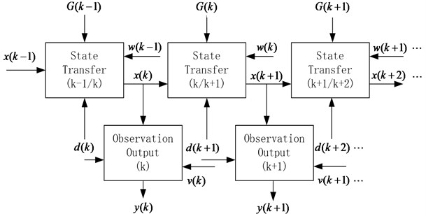
The state estimation and observation processes of the discrete system of the 6-state variables and 2-output variables are illustrated in Fig. 1.
Fig. 1State estimation and observation processes of the suspension system
3. Analysis for KF and MME algorithm
3.1. KF algorithm for road profile estimation
Based on Section 2, the problem of optimal estimation of can be solved by minimization of the loss function [20]:
where represents the prediction of , and represents the prior estimation of . Details of the loss function can be found in [20].
A recursive estimation form of may be expressed as:
where denotes the prediction of , and is the KF gain. The difference between and is called the filter innovation at the th step. Assuming that the prior estimation and the current observation are Gaussian random variables, the optimal solution to the problem is given by the following procedure [20, 21]:
Initialization:
• The initial state and covariance are expressed as:
Time update:
• The prediction of the state and covariance are computed as:
Measurement update:
• The filter gain is determined as:
• The state estimation is deduced as:
• The estimated covariance is calculated as:
where denotes the transpose of a vector.
Based on the analysis above, the recursive form of the road profile estimation at the step may be given as:
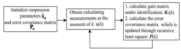
where is the correction parameter in the estimation. Combining Eq. (10) and Eq. (14), the flow chart of KF is given in Fig. 2.
Fig. 2The flow chart of the KF algorithm
3.2. MME theory representation
The MME approach solves the system error model under the covariance constraint of the observation Eq. (16). The objective function of the MME compensator is expressed as [23, 26]:
where represents the weight matrix of , and is estimated using the last time step, and can be expressed as:
where represents the Jacobi matrix of the observation equation; and are the 1st Lie derivations of about and , and are calculated as:
Using the minimum value principle, based on MME, the optimal sprung mass error can be given as:
The key of the MME criterion estimation is to properly choose the weight matrix . It can be expressed as:
where is the time scale for approaching .
Remark: It is difficult to choose in practice. Due to the unpredictable white Gauss measurement noise, an ideal is strongly time-dependent, unpredictable and even negative definite [26]. Such a result was adopted here, i.e. was chosen as a constant.
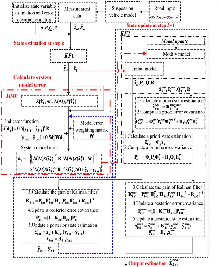
Fig. 3The flow chart of the estimation process based on MME criterion and KF algorithm
3.3. KF algorithm based MME criterion
The chart of the proposed algorithm in this paper is depicted in Fig. 3. The Fig. 3 can be described as follows. First, the initial data, i.e. system covariance matrix, measurement data etc., are obtained from suspension system. Second, the error of suspension system is calculated using MME criterion after acquiring state estimation at step . Then, combining the MME&KF algorithms, the state at step is updated to new state at . Finally, the estimated information for the road profile at the new step is used as the initial state for the following step. Further details can be found in [23].
As shown in Fig. 3, the integrated estimation MME&KF approach tries to provide a more accurate suspension state estimation.
According to Eq. (6) and Eq. (7), the KF estimation algorithm for the discrete system may be summarized as:
where , and are considered the optimal estimated vector and error covariance matrix of former time step; is the KF gain matrix; is unit matrix.
The estimation process from to detailed in Eq. (21) requires three types of information, i.e., the current input and observation information; the estimation results of the last step; and the system and measurement statistical information. Finally, the estimation returns the KF gain, system state and error covariance matrix for the current step.
4. Analysis for simulation and test
4.1. Simulation results and analysis
In this work, we applied the MME&KF algorithm to estimate the state of the road profile for a suspension system. The ISO Level-B, ISO Level-C and ISO Level-D were taken as examples to illustrate the method. Also, the ISO level-B, ISO Level-C and ISO Level-D were calculated and used as the road excitation [29]. Note that it was assumed the tire did not lose contact with the ground [36-40].
The estimation accuracy of the MME&KF method proposed in this work was compared to the performance of KF under ISO level-B, ISO Level-C and ISO Level-D road excitations. Details are shown as follows.
4.1.1. Case 1: ISO level-B excitation simulation
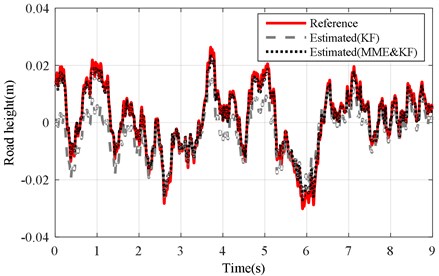
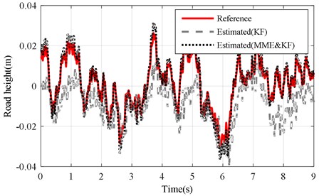
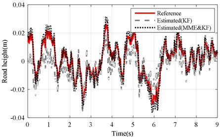
The results for the simulation configuration based on an unchanged sprung mass are also illustrated under ISO level-B excitation in Fig. 4. Second, an additional body load (180 kg) was studied [36] under ISO level-B excitation in Fig. 5.
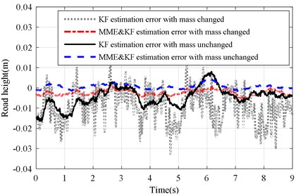
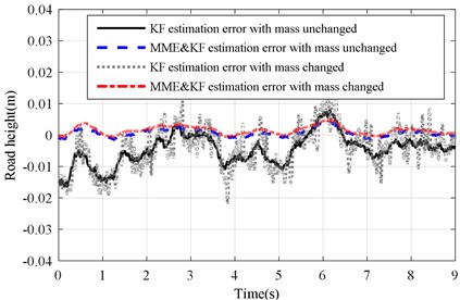
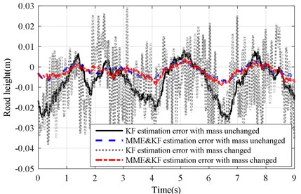
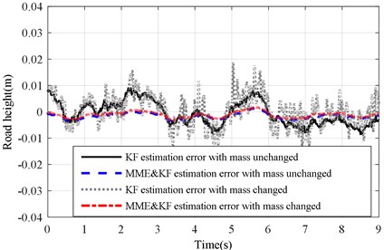
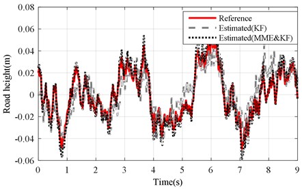
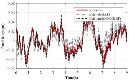
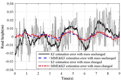
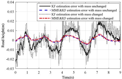
Figs. 5(a) and (b) illustrate the corresponding results of the KF and MME&KF results. Fig. 6(a) and (b) show the estimation error of the road profile for a varying sprung mass under the KF and MME&KF algorithms.
From Figs. 6(a) and (b), we can see that the estimation error of KF clearly fluctuates as the sprung mass changed under Level-B road excitation, and the MME&KF approach can improve the accuracy of the road profile for a varying sprung mass (model error).
Fig. 4Results of road level-B excitation (vveh= 40 km/h): road profile estimation of KF and MME&KF with mb unchanged (mb=mb)
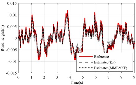
Fig. 5Road profile comparison results of mb changed under road level-B excitation (vveh= 40 km/h)
a) KF and MME&KF achieved with altered ()
b) KF and MME&KF achieved with altered ()
4.1.2. Case 2: ISO level-C excitation simulation
The estimation accuracy of the MME&KF method proposed in this work was compared to the performance of the KF under ISO level-C excitation. The results for the simulation configuration based on an unchanged sprung mass are also illustrated under ISO level-C excitation in Fig. 7. Second, an additional body load (180 kg) was studied [36] under ISO level-C excitation in Fig. 8.
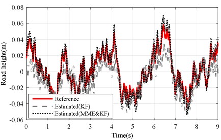
The corresponding results of the KF and MME&KF methods are illustrated in Fig. 7 and show that the higher estimation accuracy can be obtained with MME&KF. Figs. 8 and 9 show the estimation error of the road profile for a varying sprung mass under the KF and MME&KF algorithms. The simulation results showed that a smaller road excitation error is obtained using the proposed method.
Fig. 6Estimation error of KF and MME&KF road profile on road Level-B at vveh= 40 km/h
a) with altered ()
b) with altered ()
Fig. 7Results of road level-C excitation (vveh= 40 km/h): road profile estimation of KF and MME&KF with mb unchanged (mb=mb)
4.1.3. Case 3: ISO level-D excitation simulation
The estimation accuracy of the MME&KF method proposed in this work was compared to the performance of the KF under ISO level-D excitation. The results for the simulation configuration based on an unchanged sprung mass are also illustrated under ISO level-D excitation in Fig. 10. Second, an additional body load (180 kg) was studied [36] under ISO level-D excitation in Fig. 11.
Fig. 8Road profile estimation results of mb changing under road level-C excitation (vveh= 40 km/h)
a) KF and MME&KF achieved with altered ()
b) KF and MME&KF achieved with altered ()
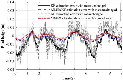
Fig. 9Estimation error of KF and MME&KF road profile on road Level-C at vveh= 40 km/h
a) with altered ()
b) with altered ()
The corresponding results of the KF and MME&KF are illustrated in Fig. 10 and show that higher estimation accuracy can be obtained for MME&KF. Figs. 11 and 12 show the estimation error of the road profile for a varying sprung mass under the KF and MME&KF algorithms. The simulation results show that a smaller road excitation error is obtained using the proposed method.
Fig. 10Results of road level-D excitation (vveh= 40 km/h): road profile estimation of KF and MME& KF with mb unchanged (mb=mb)
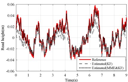
Fig. 11Road profile estimation results of mb changing under road level-D excitation (vveh= 40 km/h)
a) KF and MME&KF achieved with altered ()
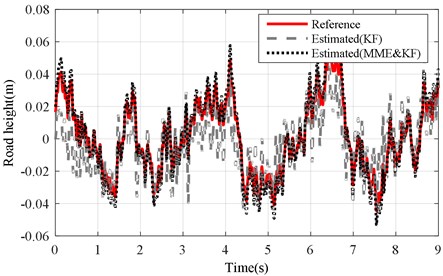
b) KF and MME&KF achieved with altered ()
In addition, the error values of the estimation standard deviation (STD) were calculated under ISO Level-B, ISO Level-C and ISO Level-D road excitation, and the simulation results are summarized in Table 2. The error of STD is higher with the KF estimation than MME&KF under the varying sprung mass.
Fig. 12Estimation error of KF and MME&KF road profile on road Level-D at vveh= 40 km/h
a) with altered ()
b) with altered ()
Table 2Calculation STD estimation values of different KF variations on road Level-B/C/D Profile at Vvel= 40 km/h
Filter state estimation | Road excitation | Filter mode | (kg) | Simulation results error STD (%) | Remarks |
ISO level-B excitation | KF | 7.3 | represents the sprung mass of vehicle; represents the changed sprung mass of vehicle | ||
MME&KF | 3.3 | ||||
KF | 7.6 | ||||
MME&KF | 3.7 | ||||
KF | 10.3 | ||||
MME&KF | 5.5 | ||||
ISO level-C excitation | KF | 8.1 | |||
MME&KF | 4.6 | ||||
KF | 9.5 | ||||
MME&KF | 5.2 | ||||
KF | 12.1 | ||||
MME&KF | 8.3 | ||||
ISO level-D excitation | KF | 10.5 | |||
MME&KF | 6.5 | ||||
KF | 12.8 | ||||
MME&KF | 7.9 | ||||
KF | 16.4 | ||||
MME&KF | 11.5 |
4.2. Experimental results and analysis
Because it is not easy to accurately obtain the time domain road profile, road profile is produced using the excitation equipment [36, 37].
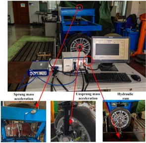
The performance estimation of the KF&MME algorithm was conducted using the available test rig for a quarter suspension system, as pictured in Fig. 13. In the road profile estimation test process, road excitation force on the wheel was measured by a hydraulic ram, and sprung and unsprung mass accelerometers were installed to acquire data from the road excitation. During the experiments, the road excitation reference signal for the estimated quantity was computed off-line using a road excitation model [28, 29] for the test rig.
The road profile estimation accuracy of the proposed MME&KF algorithm was compared to the performance of the KF.
Fig. 13Quarter vehicle suspension test rig for road profile estimation
4.2.1. Case 1: ISO level-B excitation measured
Based the same simulation environment, the experimental and simulation results were compared and summarized in Figs. 14 and 15 under Level-B road excitation.
Fig. 14Road profile results of measured KF and MME&KF estimation on road Level-B at vveh= 40 km/h with mb unchanged (mb=mb)
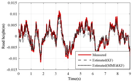
Figs. 15(a) and (b) illustrate the test and estimation results of KF and MME&KF methods. Figs. 16(a) and (b) show the estimation error of the test road profile for a varying sprung mass under the KF and MME&KF algorithms. The worst estimation accuracy occurred when using the KF algorithm under the varying sprung mass condition, but higher estimation accuracy can be obtained using the MME&KF algorithm under both changing and without changing conditions. This demonstrates that the proposed MME&KF method is most effective under both the varying and without changing sprung mass conditions.
Fig. 15Road profile results of mb changed under road level-B excitation (vveh= 40 km/h)
a) KF and MME&KF achieved with altered ()
b) KF and MME&KF achieved with altered ()
Fig. 16Estimation error of KF and MME&KF road profile on road Level-B at vveh= 40 km/h
a) with altered ()
b) with altered ()
4.2.2. Case 2: ISO level-C excitation measured
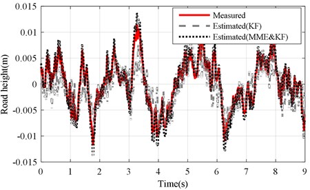
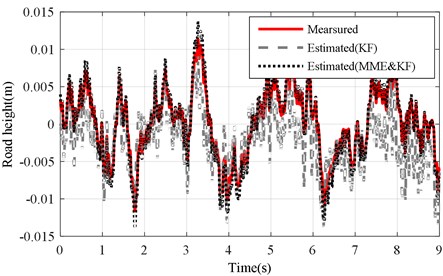
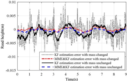
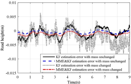
The same experiment was performed under the Level-C road excitation. Results of the two estimation methods were compared and summarized in Figs. 17-19 under the Level-C road excitation. Fig. 17 shows the test and estimation results of the KF and MME&KF approaches. Figs. 18 and 19 illustrate that higher estimation accuracy can also be acquired using MME&KF algorithm under a changing and unchanging sprung mass under Level-C excitation conditions, and the proposed MME&KF algorithm is more effective than using only the KF algorithm.
Fig. 17Road profile results of measured KF and MME&KF estimation on road Level-C at vveh= 40 km/h with mb unchanged (mb=mb)
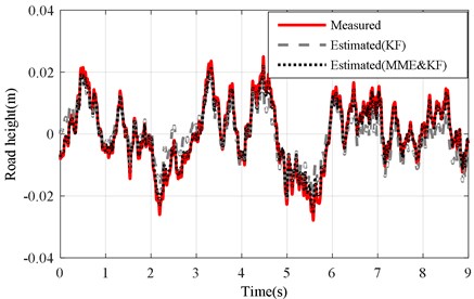
Fig. 18Road profile results of mb changed under road level-C excitation (vveh= 40 km/h)
a) KF and MME&KF achieved with altered ()
b) KF and MME&KF achieved with altered ()
Fig. 19Estimation error of KF and MME&KF road profile on road Level-C at vveh= 40 km/h
a) with altered ()
b) with altered ()
4.2.3. Case 3: ISO level-D excitation measured
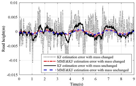
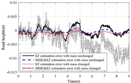
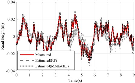
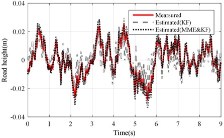
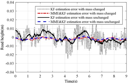
The same experiment was performed under the Level-D road excitation. Results of the two estimation methods were compared and summarized in Figs. 20-22. Fig. 20 shows the test and estimation results of the KF and MME&KF approaches. Figs. 21 and 22 illustrate that higher estimation accuracy can be obtained using the MME&KF algorithm under a varying sprung mass or unchanging sprung mass under Level-D excitation conditions, and the proposed MME&KF algorithm is more effective than using only the KF algorithm.
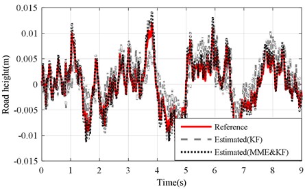
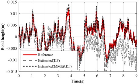
Fig. 20Road profile results of measured KF and MME&KF estimation on road Level-D at vveh= 40 km/h with mb unchanged (mb=mb)
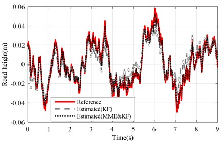
Fig. 21Road profile results of mb changed under road level-D excitation (vveh= 40 km/h)
a) KF and MME&KF achieved with altered ()
b) KF and MME&KF achieved with altered ()
Fig. 22Estimation error of KF and MME&KF road profile on road Level-D at vveh= 40 km/h
a) with altered ()
b) with altered ()
Moreover, the test error values of the STD are listed in Table 3. The error values of the estimation STD were calculated, and the test results are presented in Table 3. Comparing them to the simulation results, the same conclusion can be obtained under the ISO Level-B, ISO Level-C and ISO Level-D road excitations.
Table 3Calculation STD estimation values of different KF variations on road Level-B/C/D Profile at Vvel= 40 km/h
Filter state estimation | Road excitation | Filter mode | (kg) | Estimation results error STD (%) | Remarks |
ISO level-B excitation | KF | 7.8 | represents the sprung mass of vehicle; represents the changed sprung mass of vehicle. | ||
MME&KF | 4.5 | ||||
KF | 8.5 | ||||
MME&KF | 4.8 | ||||
KF | 12.5 | ||||
MME&KF | 6.8 | ||||
ISO level-C excitation | KF | 9.2 | |||
MME&KF | 5.8 | ||||
KF | 11.5 | ||||
MME&KF | 7.8 | ||||
KF | 15.4 | ||||
MME&KF | 9.6 | ||||
ISO level-D excitation | KF | 13.5 | |||
MME&KF | 8.5 | ||||
KF | 16.8 | ||||
MME&KF | 10.9 | ||||
KF | 18.4 | ||||
MME&KF | 14.5 |
Based on the analysis above, it can be seen that the estimation data from the MME&KF are closer to the measurement data. It may be concluded that more accurate road profile estimations can be achieved by employing the MME&KF algorithm. It should be noted that because the nonlinear tire characteristics are not considered during the process of road profile estimation; this may lead to a road profile estimation error under varying conditions of the tire.
5. Conclusions
In this paper, a new approach combining the MME criterion and a KF algorithm was proposed to estimate the road profile for a vehicle suspension system. Using the proposed method, a higher accuracy of the road profile for the suspension system can be obtained, enabling the analysis of road information. The main conclusions are as follows:
1) Based on the road excitation model, the influences of sprung mass variations on road profile observer performance can be studied. Results showed that the traditional KF did not obtain satisfactory accuracy under this condition.
2) The MME&KF algorithm was proposed to improve the estimation accuracy of the road profile under various sprung masses and ISO Level-B, ISO Level-C and Level-D road excitations.
Finally, the simulation and experimental results showed that the proposed MME&KF algorithm obtains a high accuracy of the state estimation for the road profile, which was validated in MATLAB and using a test rig under ISO level-B and ISO level-C road excitations. The STD estimation error of road profile is no more than 10 % and the STD estimation error of the road profile is no more than 19 % under ISO level-D road excitation.
In the future, the nonlinear quarter suspension model will be used directly and the proposed method will be applied to the full-car road profile estimations.
References
-
Cao D., Song X., Ahmadian M. Editors’ perspectives: road vehicle suspension design, dynamics, and control. Vehicle System Dynamics, Vol. 49, Issues 1-2, 2011, p. 3-28.
-
Martinez J. C. T., Fergani S., Sename O., et al. Adaptive road profile estimation in semiactive car suspensions. IEEE Transactions on Control Systems Technology, Vol. 23, Issue 8, 2015, p. 2293-2305.
-
Qin Y., Dong M., Zhao F., et al. Road profile classification for vehicle semi-active suspension system based on adaptive neuro-fuzzy inference system. IEEE Control Decision Conference, Osaka, Japan, Vol. 1, Issue 1, 2015, p. 1538-1543.
-
Poussot-Vassal C., Sename O., Dugard L. Attitude and handling improvements based on optimal skyhook and feedforward strategy with semi-active suspensions. International Journal of Vehicle Autonomous Systems, Special Issue on Modeling and Simulation of Complex Mechatronic Systems, Vol. 6, Issues 3-4, 2008, p. 308-329.
-
Lee J. H., Lee S. H., Kang D. K., et al. Development of a 3D road profile measuring system for unpaved road severity analysis. International Journal of Precision Engineering and Manufacturing, Vol. 18, Issue 2, 2017, p. 155-162.
-
Doumiati M., Victorino A., Charara A., et al. Estimation of road profile for vehicle dynamics motion: experimental validation. American Control Conference, San Francisco, CA, USA, Vol. 1, Issue 1, 2011, p. 5237-5242.
-
Mccann R., Nguyen S. System identification for a model-based observer of a road roughness profiler. IEEE Region 5th Technical Conference, Fayetteville, USA, Vol. 1, Issue 1, 2007, p. 336-343.
-
Zhang Z. Z., Deng F., Huang Y., et al. Road roughness evaluation using in-pavement strain sensors. Smart Materials and Structures, Vol. 24, Issue 11, 2015, p. 115029.
-
Rath J., Veluvolu K., Defoort M. Simultaneous estimation of road profile and tire road friction for automotive vehicle. IEEE Transaction on Vehicular Technology, Vol. 64, Issue 58, 2015, p. 4461-4471.
-
Ngwangwa H. M., Heyns P. S., Breytenbach H. G. A., et al. Reconstruction of road defects and road roughness classification using artificial neural networks simulation and vehicle dynamic responses: application to experimental data. Journal of Terramechanics, Vol. 53, Issue 5, 2014, p. 1-18.
-
Qin Y., Langari R., Gu L. The use of vehicle dynamic response to estimate road profile input in time domain. ASME Dynamic System Control Conference, San Antonio, USA, 2014.
-
Yousefzadeh M., Azadi S., Soltani A. Road profile estimation using neural network algorithm. Journal of Mechanical Science and Technology, Vol. 24, Issue 3, 2010, p. 743-754.
-
Fauriat W., Mattrand C., Gayton N., et al. Estimation of road profile variability from measured vehicle responses. Vehicle System Dynanics, Vol. 54, Issue 5, 2016, p. 585-605.
-
Gonzalez A., O’brien E. J., Cashell K. The use of vehicle acceleration measurements to estimate road roughness. Vehicle System Dynamics, Vol. 46, Issue 5, 2008, p. 483-499.
-
GÖhrle C., Schindler A., Wagner A. Road profile estimation and preview control for low-bandwidth active suspension systems. IEEE/ASME Transactions on Mechatronics, Vol. 20, Issue 5, 2015, p. 2299-2310.
-
Li Z. J., Kolmanovsky I. V., Atkins, E. M., et al. Road disturbance estimation and cloud-aided comfort-based route planning. IEEE Transactions on Cybernetics, 2016, p. 1-13.
-
Tudón Martínez J.-C., Fergani S., Sename O., et al. Adaptive road profile estimation in semi-active car suspensions. IEEE Transactions on Control Systems Technology, Institute of Electrical and Electronics Engineers, Vol. 23, Issue 6, 2015, p. 2293-2305.
-
Imine H., Delanne Y., M’Sirdi N. K. Road profile input estimation in vehicle dynamics simulation. Vehicle System Dynanics, Vol. 44, Issue 3, 2006, p. 285-303.
-
Qin Y., Langari R., Wang Z., et al. Random road profile estimation using adaptive Kalman filter and adaptive super-twisting observer. American Control Conference, Seattle, US., 2017.
-
Kalman R. E. A new approach to linear filtering and prediction problem. Journal Fluids English, Vol. 82, Issue 2, 1960, p. 35-45.
-
Lindgärde O. Kalman filtering in semi-active suspension control. Proceedings of the 15th Triennial World Congress, Vol. 1, Issue 1, 2002, p. 1-6.
-
Xu D. D., Xiao Z., Li D. P., et al. Optimization of parallel algorithm for Kalman filter on CPU-GPU heterogeneous system. 12th International Conference on Natural Computation, Fuzzy Systems and Knowledge Discovery, Vol. 1, Issue 1, 2016, p. 1-8.
-
Mook D. J., Junkins J. L. Minimum model error estimation for poorly modeled dynamic systems. Journal of Guidance Control and Dynamics, Vol. 11, Issue 5, 1988, p. 256-26.
-
Crassidis J. L., Markley F. L. Minimum model error approach for attitude estimation. Journal of Guidance Control and Dynamics, Vol. 20, Issue 8, 1997, p. 1241-1247.
-
Lin Y., Deng Z. Minimum model error approach for attitude estimation. Journal of Harbin Institute Technology, Vol. 34, Issue 3, 2002, p. 14-18.
-
Liu W., He H., Sun F. Vehicle state estimation based on minimum model error criterion combing with extended Kalman filter. Journal of Franklin Institute, Vol. 353, Issue 4, 2016, p. 834-856.
-
Qin Y. C., Langari R., Wang Z. F., et al. Road excitation classification for semi-active suspension system with deep neural networks. International Journal of Fuzzy Systems, 2017, accepted.
-
Wang Z. F., Dong M. M., Qin Y. C., et al. Suspension system state estimation using adaptive Kalman filtering based on road classification. Vehicle System Dynamics, Vol. 55, Issue 3, 2016, p. 371-398.
-
Mechanical Vibration-Road Surface Profiles-Reporting of measured data. ISO8601-1995, 1995.
-
Yu W., Zhang X., Guo K., et al. Adaptive Real-Time estimation on road disturbance properties considering load variation via vehicle vertical dynamics. Mathematical Problems in Engineering, 2013, https://doi.org/10.1155/2013/283528.
-
Sun W., Pan H., Zhang Y., et al. Multi-objective control for uncertain nonlinear active suspension systems. Mechatronics, Vol. 24, Issue 5, 2014, p. 318-327.
-
Qin Y. C., Zhao F., Wang Z. F., et al. Comprehensive analysis influence of controllable damper time delay on semi-active suspension control strategies. Journal of Vibration and Acoustics, Vol. 139, 2017, p. 2017-3.
-
Zhao F., Ge S. S., Tu F. W., et al. Adaptive neural network control for active suspension system with actuator saturation. IET Control Theory and Application, Vol. 10, Issue 14, 2016, p. 1696-1705.
-
Qin Y. C., Dong M. M., Langari R., et al. Adaptive hybrid control of vehicle semi-active suspension based on road profile estimation. Shock and Vibration, 2015, https://doi.org/10.1155/2015/636739.
-
Qin Y. C., Xiang C. L., Wang Z. F., et al. Road excitation classification for semi-active suspension system based on system response. Journal of Vibration and Control, 2017, https://doi.org/10.1177/1077546317693432.
-
Pletschen N., Klaus J. Diepold Nonlinear state estimation for suspension control applications: a Takagi-Sugeno Kalman filtering approach. Control Engineering Practice, Vol. 61, 2017, p. 292-306.
-
Mahyuddin M. N., Na J., Herrmann G., et al. Adaptive observer-based parameter estimation with application to road gradient and vehicle mass estimation. IEEE Transactions on Industrial Electronics, Vol. 61, Issue 6, 2014, p. 2851-2863.
-
Rath J. J., Veluvolu K. C., Defoort Simultaneous M. Estimation of road profile and tire road friction for automotive vehicle. IEEE Transactions on Vehicular Technology, Vol. 64, Issue 10, 2015, p. 4461-4471.
-
Wang Z. F., Dong M. M., Zhao W. P., et al. A novel tread model for tire modelling using experimental modal parameters. Journal of Vibroengineering, Vol. 19, Issue 2, 2017, p. 1225-1240.
-
Wang Z. F., Dong M. M., Gu L., et al. Influence of road excitation and steering wheel input on vehicle system dynamic responses. Applied Science, Vol. 7, Issue 6, 2017, p. 570.
Cited by
About this article

This work was supported by the National Natural Science Foundation of China (Grant No. U1564210), Innovative Talent Support Program for Post-Doctorate of China (Grant No. BX201600017) and China Postdoctoral Science Foundation (Grant No. 2016M600934).
