Abstract
Because of various advantages of planetary transmission system, it has been widely used in modern industry. And study on planetary gearbox degradation feature analysis method has important significance for mechanical system prognostics and health management (PHM). In order to analysis the degradation characteristic of planetary gearbox, Energram is proposed in this paper based on Kurtogram. Kurtogram is used for finding the optimal frequency band to rotating machinery fault diagnosis by calculating kurtosis. Similarly, Energram is used to show the energy trend of each frequency band by calculating energy, and arithmetic Energram is used to show the change of frequency band energy. The principle and application of Energram and arithmetic Energram are described by experimental data examples in this paper. A detailed study of planetary gearbox degradation characteristics is expressed in case study, which including Energram, arithmetic Energram and four particular comparative analyses. And the conclusions of each comparative analysis are given.
1. Introduction
As the advantages of strong load-bearing capacity, large transmission ratio, etc., planetary transmission systems are widely used in complex mechanical equipment, such as wind turbine, helicopters and heavy trucks. Once planetary transmission systems severe degradations occur they may cause machines to malfunction and even fail, which leads to financial losses and even fatal incidents. Moreover, planetary transmission system significantly differs from fixed-axis transmission system because of its unique structure [1, 2]. As a result, it is very important to research on health state assessment method and degradation analysis approach of planetary transmission systems.
Health state evaluation of planetary transmission system is a hot research topic in recent years, many scholars study on this aspect. For example, Chaari [3, 4] investigated the effects of planetary gearbox gear fault on vibration responses through dynamics modeling and analysis. In order to calculate both local and distributed fault frequencies, Feng and Zuo [5] proposed planetary gearbox vibration signal models and deprived equations. Considering the working environment of wind turbines was easy to change, Chen and Feng [2, 6] studied on planetary gearbox fault diagnosis and condition monitoring methods under nonstationary conditions. Lei [7] and Bartelmus [8, 9] respectively put forward feature indices for planetary gearboxes condition monitoring under constant and nonstationary operations. Some transmission systems have more than primary planet gears, Lei [10, 11] researched on health condition identification of multi-stage planetary gearboxes. He also summarized the research and development of planetary gearboxes condition monitoring and fault diagnosis [12].
Some scholars have focused on the degradation analysis and fault prediction of planetary gearbox. For instance, Marcos and George [13] investigated the prediction of axial crack growth in an UH-60 planetary carrier plate. Cheng and Hu [14, 15] researched on pitting damage level estimation and quantitative damage detection of planetary gear sets based on simulations and physical models. Ni [16] used state-space model to estimate remaining useful life of planetary gearbox. In general, the degradation analysis of planetary transmission system research is just started, and it needs future study.
If mechanical transmission system occur fault, system tends to produce a series of shock pulse signals in the running process. And the shock pulse signals become the key to fault diagnosis for the mechanical transmission system. Since Stewart [17] put forward the concept of kurtosis, it has been as an important index to reflect mechanical part health states. And then the Spectral Kurtosis (SK) concept was proposed, which can be used to determine the optimal frequency band for shock pulse signal component based on kurtosis. Antoni [18, 19] went into details of the definition and calculation method of SK, and applied SK to bearing fault diagnosis. He also proposed two methods to calculate SK, the first one was based on short time Fourier transform (STFT), and the other is based on 1/3 binary filter banks [20]. Then, Lei [21] proposed a new method to build Kurtogram, which used wavelet packet decomposition (WPD) to replace the STFT in extracting transient characteristics and calculated the temporal signal kurtosis filtered by WPD. Barszcz and Jablonski [22] used the kurtosis of the envelope spectrum for the demodulated signal to determined frequency band, rather than the kurtosis of the filtered time signal, and this approach was named Protrugram. Wang [23] developed Protrugram to an enhanced Kurtogram. Wang and Liang [24] established a theoretical model of multiple bearing faults and developed a multi-fault diagnosis method based on adaptive spectral kurtosis analysis. In order to quickly determine the resonant frequency bands, Tse and Wang [25] put forward a new method named Sparsogram. Using kurtosis value to estimate the strength of cyclical shocks pulse signal was defective, it leaded to the determined optimal band might be not accurate sometime. Faced with this shortcoming, Zhang [26] and McDonald [27] used correlated kurtosis (CK) to replace kurtosis to solve the problem and applied this approach in fault diagnosis of bearing and gearbox. Obviously, the SK and based on its various methods have been widely used in the fault diagnosis of rotating machinery.
SK and its improved methods also used in rotating machinery degradation analysis. Faris [28-30] studied in detail the application of SK in bearing faults detection and naturally degradation detection. And he compared to the effectiveness of four algorithms (least mean square (LMS), linear prediction, SK and fast block LMS) in bearing detection. Lotfi [31] investigated skidding in wind turbine high-speed shaft bearings degradation for run-to-failure testing using squared envelope analysis based on SK. Huang [32] put forward a feature extraction method that combines Blind Source Separation (BSS) and SK to separate independent noise sources and used this method in bearing incipient degradation analysis. However, the research on SK and its improved methods for rotating machinery degradation analysis is still not much.
This paper puts forward a new improved Kurtogram method to analysis degradation process of planetary gearbox. In the proposed method, Energy is calculated rather than the kurtosis in the running process of Kurtogram. The frequency-domain graphs of each time point in degradation process are composed of a time-domain diagram, which is named Energram. And the characteristics of system degradation process can be extracted from Energram.
The main contributions of this study are: (a) Energram is put forward based on Kurtogram, degradation characteristic index (namely energy) are decomposed from frequency domain and time domain at the same time. As a result, Energram can not only observe energy distribution of different frequency band within a certain time interval, but also can analyze energy trend over time of a certain frequency band. This method extends the traditional analysis approach of degradation feature index from 2-domain to 3-domain. And the degradation information extraction means become richer. (b) Arithmetic Energram is proposed in this paper, the change of energy in arithmetic period is calculated on the basis of Energram. Arithmetic Energram shows the change of all frequency band energies, and the relationship between total energy trend (increase or decrease) and the change of different frequency band energy can be found.
The remainder of this paper is organized as follows. Section 2 is devoted to the basic principle and application of Kurtogram. Section 3 studies the proposed methods, Kurtogram and arithmetic Energram. The degradation characteristics of planetary gearbox are detail analyzed in Section 4. And conclusions are made in Section 5.
2. Spectral kurtosis and Kurtogram
It is critical to grasp the basic principle of SK for its application in fault diagnosis. This article will describe the basic theory of SK and Kurtogram, and illustrate their application by examples using open experimental data.
According to Wold-Cramer representation, any stochastic nonstationary process can be decomposed into a causal, linear and time-varying system [20, 33]:
where is the complex envelope of (the time varying transfer function of the system) at frequency , and is a spectral increment. Then, the SK can be clearly expressed as the fourth-order normalized [20, 33]:
where the 2-order spectral moments are expressed as:
Spectral cumulants of order have the interesting property that is non-zero for non-Gaussian processes.
In general, the vibration signal corrupted with noise, , is stationary noise. And SK can be described by:
where is the noise-to-signal between and :
Moreover, when is a stationary Gaussian noise independent of , the SK can be simplified as:
It is not difficulty to found that the basic idea behind the SK is to get a high value when the signal is transient, and will be zero when the signal is stationary Gaussian [34].
Antoni [20] proposed SK on the basis of a series of digital filtering, and he made detailed research on it. The mainly harvest in computing speed is the SK calculation method based on binary decomposition, which is very similar with the FFT algorithm. In the calculation algorithm, the frequency bandwidth is equal to half of the frequency bandwidth in previous stage. And the calculation algorithm is known as binary tree. Moreover, there is also a 1/3-binary tree, all combinations of center frequency and bandwidth for the 1/3-binary tree Kurtogram are shown in Fig. 1 and Table 1 ( is the signal sampling frequency).
Take bearing failure data of Case Western Reserve University (CWUR) as an example to illustrate the application of Kurtogram method. The test bearing with 7 mils single point fault in bearing outer raceway located 6 o’clock position. The test stand speed is 1730 rpm and load is 3 hp. The sampling frequency is 12 kHz and the Nyquest frequency is 6000 Hz. According to experience, the signal components within 30 times rotating frequency are mainly frequency components generated by shaft and gear, which tends to be ignored in analysis. Therefore, this paper only analysis the frequency band in range [1000, 6000] Hz. The SK is calculated by 1/3-binary tree Kurtogram and the output Kurtogram is shown in Fig. 2. It is easy to find the optimum resonance frequency band in 6-th level, and the frequency band interval is [3083.5, 3500.2] Hz. Then, envelope analysis of signal within [3083.5, 3500.2] Hz is implemented to check fault characteristic frequency of bearing outer ring. The outer ring fault feature frequency (BPFO) is obviously in Fig. 3. As a result, Kurtogram is effective for fault diagnosis.
Table 1Frequency map of the 1/3-binary tree Kurtogram
Levels | Frequency bandwidth (Hz) | Number of frequency bands | |
0 | 0 | /2 | 1 |
1 | 1 | /4 | 2 |
2 | 1.6 | /6 | 3 |
3 | 2 | /8 | 4 |
4 | 2.6 | /12 | 6 |
5 | 3 | /16 | 8 |
6 | 3.6 | /24 | 12 |
7 | 4 | /32 | 16 |
Fig. 1Combinations of center frequency and bandwidth for the 1/3-binary tree Kurtogram estimator
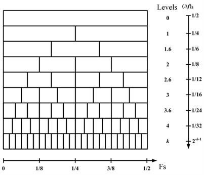
Fig. 2Kurtogram of bearing outer race fault
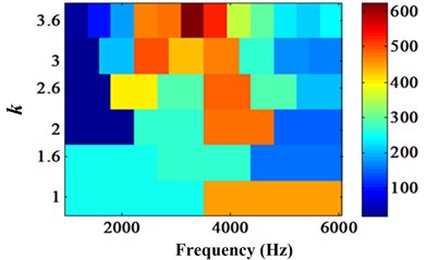
Fig. 3Envelope spectrum of [3083.5, 3500.2] Hz
![Envelope spectrum of [3083.5, 3500.2] Hz](https://static-01.extrica.com/articles/18129/18129-img3.jpg)
3. Energram and arithmetic Energram
3.1. Energram
Previous studies have shown that kurtosis can be effective used in rotating machinery fault diagnosis. Meanwhile, energy can rise gradually as system degradation increase and it has been widely used in rotating machinery degradation research.
The idea of Energram is put forward based on Kurtogram. In order to reflect the system degradation degree, energy is calculated as the characteristic index instead of kurtosis. In Kurtogram method, kurtosis is extracted (as shown in Eq. (7)) after the frequency bands decomposed. Similarly, energy is calculated as Eq. (8) in Energram. As a result, the Energram method can be used for degradation research. The flow chart of Energram method is presented in Fig. 4:
where is discrete vibration signal of the time series over the time interval [1, ], and is the mean value of discrete vibration signals.
Fig. 4Flow chart of Energram
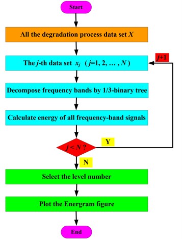
Fig. 5Flow chart of arithmetic Energram
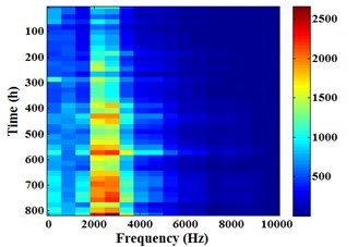
Take the second group of Intelligent Maintenance Systems Center (IMS) bearing life-cycle data as an example to illustrate the generation process of Energram. This group of bearing whole life data is a total of 984 set data, and the sampling frequency is 20 kHz for duration of 1.024 seconds, namely 20 kHz.
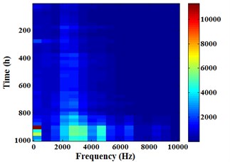
The Energram of the 850th set of data is shown in Fig. 6. According to Table 1, the frequency domain [0, /2] is divided into 16 groups of frequency bands at the 7th level, and the frequency bandwidth is 625 Hz. Extracting all the 7th level Energram of the (850-984)th set of data to form a new Energram as shown in Fig. 8. The data set interval -axis is 3. Fig. 7 is the total energy of the (850-984)th set of data. Contrast Fig. 7 and Fig. 8, it can be found that Energram color depth is changing along with the change of bearing total energy, and the energy is mainly concentrated in frequency band [625, 1250] Hz.
3.2. Arithmetic Energram
In general, system runs the longer, degradation degree is the larger, and mean vibration signal energy is the higher. However, as the energy value will fluctuate, not every energy value is absolute growth.
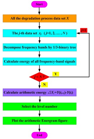
The system total running time is is the system energy at running time , the interval time , the energy difference between and is , namely is the energy increment during . As the energy is not absolute growth, may be greater than zero and may also be less than zero. Of course, is greater than zero in most cases. The flow chart of arithmetic Energram method is presented in Fig. 5.
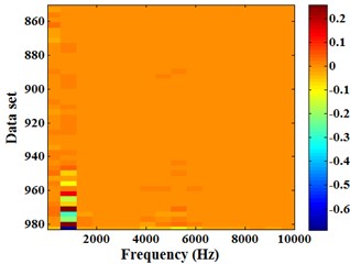
The arithmetic Energram of the (850-984)th set of data is shown in Fig. 9. It can be found that the arithmetic Energram color changes only when total energy fluctuates is intense, and the energy fluctuation is also mainly focused on frequency band [625, 1250] Hz.
Fig. 6Energram of the 850th set of data
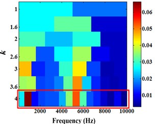
Fig. 7Total energy of the (850-984)th set of data
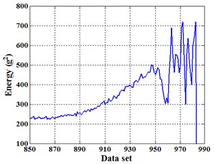
Fig. 8Energram of the (850-984)th set of data
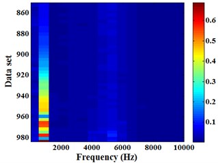
Fig. 9Arithmetic Energram of the (850-984)th set of data
4. Planetary gearbox degradation analysis
A case study of planetary gearbox degradation process is carried out to validate the effectiveness of the proposed method.
4.1. Planetary gearbox degradation experiment
The degradation process data of planetary gearbox is collected from a life-cycle experiment. The planetary gearbox experiment rig is shown in Fig. 10. The experiment rig consists of a test planetary gearbox, a drive motor, a speed and torque sensor, and a magnetic powder brake. The test gearbox is a one-stage planetary gearbox, as shown in Fig. 11 and Fig. 12, it comprises one ring gear, three planet gears and one sun gear. The gear parameters of single stage planetary gearbox are listed in Fig. 12 and Table 2.
In the life-cycle experiment, the input speed of planetary gearbox is about 1005 rpm (as shown in Fig. 13), the load provided by magnetic powder brake is about 340 Nm, and the vibration signal sampling frequency is 20 kHz for duration of 12 seconds. There are four accelerometers fitted onto the casing of planetary gearbox to record vibration signal, as shown in Fig. 11. The total experimental time is 1003 hours. As shown in Fig. 14, the abrasions of gears are very obvious after experiment.
Table 2Gear parameters of single stage planetary gearbox
Gear | Sun gear | Ring gear | Planet gear | Planet gear number |
Teeth number | 13 | 146 | 64 | 3 |
Fig. 10Planetary gearbox experiment rig
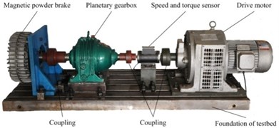
Fig. 11Mounted location of sensors
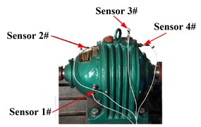
Fig. 12Schematic map of gearbox structure
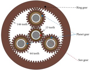
Fig. 13The input speed of planetary gearbox
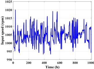
Fig. 14Gears after experiment
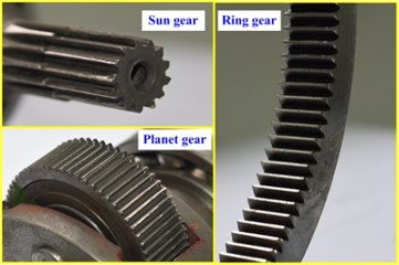
Fig. 15Energy trend of sensor 1# and 3#
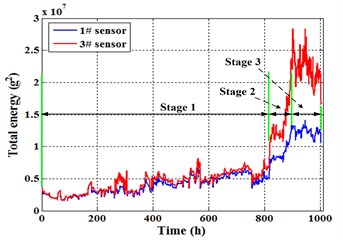
This article takes the vibration signals of sensor 1# and 3# as representatives to analyze and contrast. The total energy trend of sensor 1# and 3# are presented in Fig. 15. It can be found from the energy trends that the degradation process of planetary gearbox shows in three stages: (a) The first stage is slowly rising stage, about 0-817 h. The energy is stable, the average growth rate of energy is very slow, and the energy fluctuation range is small. (b) The second stage is rapidly rising stage, about 818-894 h. The mean growth rate of energy is obvious, there are even suddenly jumped rising phenomenon. (c) The third stage is intense fluctuation stage, about 895-1003 h. Energy changes have no fixed pattern, but fluctuates up and down of energy is quickly and the fluctuation range is large.
As shown in Fig. 15, in the first stage, the energy trends of sensor 1# and 3# is exactly similar, numerical difference is small and contact ratio is high. In the second stage, the energy increase speed of sensor 3# is much larger than sensor 1#, there are no longer overlap between the energies of sensor 1# and 3#. In the third stage, the energy fluctuation range of sensor 3# is also much larger than sensor 1#, the phenomenon shows that the energy of sensor 3# instantaneous increase and reduce is very obvious.
4.2. Energram analysis
4.2.1. Energram of sensor 1#
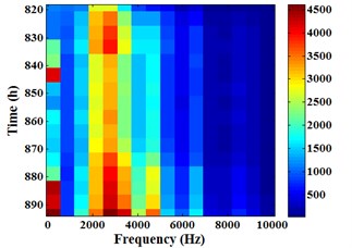
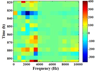
Fig. 16 is the Energram of sensor 1#. And Fig. 16(a) is the Energram for whole degradation process (0-1003 h), the y-axis time interval is 25 h. Fig. 16(b) is the Energram for the first stage (0-817 h), 20 h. Fig. 16(c) is the Energram for the second stage (818-894 h), 5 h. Fig. 16(d) is the Energram for the third stage (895-1003 h), 5 h.
Fig. 16Energram of sensor 1#
a) 0-1003 h
b) 0-817 h
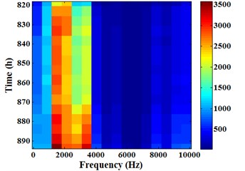
c) 818-894 h
d) 895-1003 h
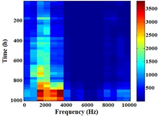
It can be found from -axis in Fig. 16 that evident color part focuses on frequency band [625, 3750] Hz. This phenomenon shows that the energy in frequency band [625, 3750] Hz is higher than other frequency bands. In the Energram for whole degradation process (Fig. 16(a)), the color in frequency band [625, 3750] Hz is more and more deeply over time. This suggests that the energy is gradually rising with running time increase. The color of last 5 in the Fig. 16(a) y-axis is most evident, and color depth fluctuates slightly. This phenomenon is completely corresponding to the third stage (the intense fluctuation stage) in energy trend.
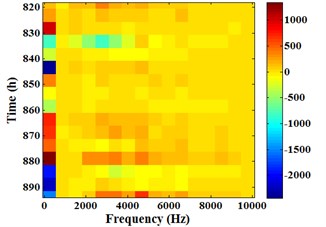
4.2.2. Energram of sensor 3#
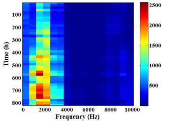
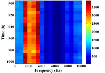
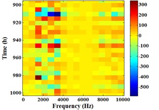
Fig. 17 is the Energram of sensor 3#, the relevant data is similar to Fig. 16. It can be found from -axis in Fig. 17 that evident color part focuses on frequency band [0, 625] Hz and [1250, 5000] Hz. This phenomenon shows that the energy is mainly distributed in frequency band [0, 625] Hz and [1250, 5000] Hz. Compared with sensor 1#, the significant difference of sensor 3# energy is the appearance in low frequency band [0, 625] Hz. Moreover, color depth changes in frequency band [0, 625] Hz is the biggest as time goes on. It shows that energy fluctuation in this frequency band is much bigger than any other frequency band in the whole degradation process.
Fig. 17Energram of sensor 3#
a) 0-1003 h
b) 0-817 h
c) 818-894 h
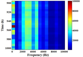
d) 895-1003 h
4.3. Arithmetic Energram analysis
4.3.1. Arithmetic Energram of sensor 1#
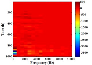
Fig. 18 is the arithmetic Energram of sensor 1# corresponding to the Energram in Fig. 16. It can be known that energy fluctuation also mainly concentrates in the frequency band [625, 3750] Hz, the major frequency bands for casing total energy fluctuation are the same to the frequency bands of main energy. Comparing the difference between Fig. 16 and Fig. 18, it is not difficult to find that the color change in time axis (-axis) of Energram is continuous and gradually deepening, but the color change in time axis of arithmetic Energram is messy and has no rules.
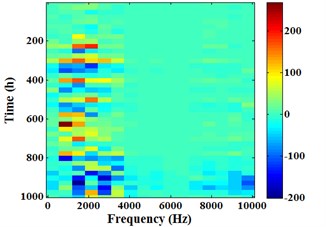
4.3.2. Arithmetic Energram of sensor 3#
Fig. 19 is the arithmetic Energram of sensor 3#. It can be found from Fig. 19(b) that the energy fluctuation in the first stage is mainly caused by the energy fluctuations in frequency band [1250, 3750] Hz. As shown in Fig. 19(c) and Fig. 19(d), it is obviously that the energy fluctuation in the second stage and the third stage is primary because of the energy fluctuations in frequency band [0, 625] Hz. The change of energy in other frequency band is much smaller. That is to say, if filter out the [0, 625] Hz signal components from original signal, the energy fluctuation range will be reduced and the energy stability characteristics will be improved.
Fig. 18Arithmetic Energram of sensor 1#
a) 0-1003 h
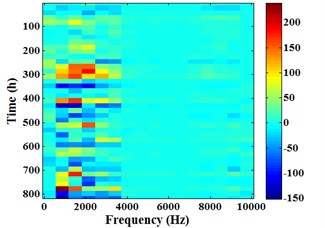
b) 0-817 h
c) 818-894 h
d) 895-1003 h
Fig. 19Arithmetic Energram of sensor 3#
a) 0-1003 h
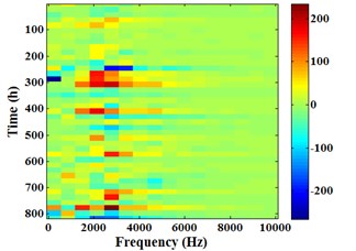
b) 0-817 h
c) 818-894 h
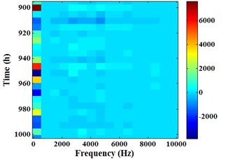
d) 895-1003 h
4.4. Comparative analysis
4.4.1. The comparison for total energy and low frequency removed energy (sensor 3#)
Total energy ([0, 10000] Hz energy), low frequency removed energy ([625, 10000] Hz energy) and low frequency energy ([0, 625] Hz energy) of sensor 3# are shown in Fig. 18. As analyzed in section 4.3.2, the energy fluctuations of sensor 3# in the second stage and the third stage is mainly caused by the energy in frequency band [0, 625] Hz. It is obviously that the energy trend of total energy and low frequency removed energy in whole degradation process (0-1004 h) is completely similar (as shown in Fig. 20(a)). As partial enlarged drawing Fig. 20(b) shown, the low frequency removed energy also has ups and downs, but the fluctuation range significantly much smaller than total energy. Moreover, the fluctuation of low frequency energy is really obvious.
Therefore, the conclusion can be obtained, in the sensor 3# position, that the vibration signal can reveal the gearbox degradation condition better after removing the low frequency noise.
Fig. 20Total energy and low frequency removed energy of sensor 3#
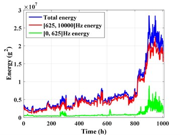
a) 0-1004 h
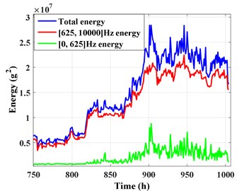
b) 750-1004 h
4.4.2. The comparison for total energy and main frequency band energy (sensor 1#)
Know by the preceding analysis in section 4.2.1, the energy of sensor 1# primarily focuses on frequency band [625, 3750] Hz. Making a comparison for total energy ([0, 10000] Hz energy), main frequency band energy ([625, 3750] Hz energy), and other frequency bands energy ([0, 625] Hz energy add to [3750, 10000] Hz energy), as shown in Fig. 21, it can be found that [625, 3750] Hz energy is much larger than the other frequency bands energy, and [625, 3750] Hz energy is close to total energy. In other words, frequency band [625, 3750] Hz indeed contains most of total energy. Although, the other frequency bands energy in the second and the third degradation stages is not small, the energy trends of [625, 3750] Hz energy is very similar to total energy in rising and fluctuation. Just like the discovery in section 4.4.1, the fluctuation range of [625, 3750] Hz energy is smaller than total energy, and [625, 3750] Hz energy is more suitable for degradation prediction.
Fig. 21Total energy and [625, 3750] Hz energy of sensor 1#
![Total energy and [625, 3750] Hz energy of sensor 1#](https://static-01.extrica.com/articles/18129/18129-img34.jpg)
Fig. 22[1250, 3750] Hz energy of sensor 1# and 3#
![[1250, 3750] Hz energy of sensor 1# and 3#](https://static-01.extrica.com/articles/18129/18129-img35.jpg)
As a result, the conclusion can be gained that main frequency band contains most of total energy. Moreover, the trends of main frequency band energy and total energy are similarly, it also can be used for degradation prediction.
4.4.3. The comparison for main frequency band energies in different sensor (sensor 1# and 3#)
As analyzed in section 4.2, the main frequency band of sensor 1# is [625, 3750] Hz and the main frequency band of sensor 3# is [1250, 5000] Hz (the low frequency band [0, 625] Hz is neglected). Take the intersection interval of main frequency bands [1250, 3750] Hz to analysis.
The energies of frequency band [1250, 3750] Hz for different sensor are shown in Fig. 22. Obviously, the energy values and energy trends of sensor 1# and 3# are so close. The only difference is that energy value of sensor 3# is a little bit more than sensor 1# in the third stage, but the energy trends and fluctuation ranges of both sensor 1# and 3# are the same. In contrast, as shown in Fig.15, the increase amplitude of sensor 3# total energy is much more than sensor 1# total energy in the second stage. And the fluctuation range of sensor 3# total energy is significantly greater than sensor 1# total energy in the third stage. These phenomena show that the energy value and the energy trend of main frequency band energy are significant difference from total energy in planetary gearbox degradation process.
Therefore, the conclusion can be obtained that the values and trend of degradation feature index (such as energy) in a specific frequency band are very close, even if the sensor position is different.
4.4.4. The comparison for total energy and different frequency band energy (sensor 1# and 3#)
According to the frequency band division method of Energram (1/3-binary tree), the frequency bands included in [1250, 3750] Hz are [1250, 1875] Hz, [1875, 2500] Hz, [2500, 3125] Hz and [3125, 3750] Hz, respectively. Extracting the energies of these frequency bands for sensor 1# and 3#, as shown in Fig. 23-26. Meanwhile, different frequency band energy of the same sensor is present in a picture, as shown in Fig. 27 and Fig. 28.
Fig. 23[1250, 1875] Hz energy
![[1250, 1875] Hz energy](https://static-01.extrica.com/articles/18129/18129-img36.jpg)
Fig. 24[1875, 2500] Hz energy
![[1875, 2500] Hz energy](https://static-01.extrica.com/articles/18129/18129-img37.jpg)
As shown in the energy trend of [1250, 1875] Hz (Fig. 23), it can be found that: (a) Although the energy fluctuation is large, there is not obvious acceleration stage in energy trend, and the energy trend in whole degradation process appears as linear. This phenomenon is closer to the physical truth of planetary gearbox degradation process. (b) Energy of sensor 1# is greater than sensor 3#, this phenomenon is inconsistent to the appearance that total energy of sensor 1# is smaller than sensor 3#. Through statistics found that a total of 4 groups of frequency bands appear this phenomenon in the 16 groups of frequency bands between [0, 10000] Hz, the other 3 groups of frequency bands are [7500, 8125] Hz, [8750, 9375] Hz and [9375, 10000] Hz, respectively.
Fig. 25[2500, 3125] Hz energy
![[2500, 3125] Hz energy](https://static-01.extrica.com/articles/18129/18129-img38.jpg)
Fig. 26[3125, 3750] Hz energy
![[3125, 3750] Hz energy](https://static-01.extrica.com/articles/18129/18129-img39.jpg)
Fig. 27Different frequency band energies of sensor 1#
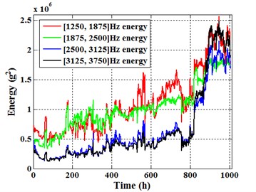
Fig. 28Different frequency band energies of sensor 3#
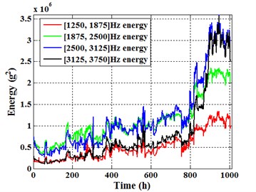
It is shown in Fig. 23-28 that, in whole degradation process, energy trend of [1250, 1875] Hz appears as linear, energy trend of [1875, 2500] Hz is between linear and three stages characteristic, energy trend of [2500, 3125] Hz appears three stages characteristic, and the three stages characteristic of [3125, 3750] Hz energy trend is the most evident. Too easy to get the conclusion, as the improvement of frequency bands in [1250, 3750] Hz, the energy trend change from linear to three stages feature, and the three stages characteristic becomes more and more clear.
As a result, the conclusions can be gained that even in the same system degradation process, the change trends of different frequency band energies also differ. In the degradation prediction, we should choose the frequency band energy that reflects the system physical deterioration process better.
5. Conclusions
As the planetary transmission system is widely used in modern industrial equipment, this paper is meant to investigate degradation feature analysis method for planetary transmission system. To this purpose, the new improved Kurtogram method (Energram and arithmetic Energram) for degradation analysis is put forward and researched. A detailed study of planetary gearbox degradation characteristics is expressed in this paper, which including Energram, arithmetic Energram and four particular comparative analyses.
The planetary gearbox degradation feature analysis based on new improved Kurtogram, which is proposed in this study, shows that Energram and arithmetic Energram can effective analysis the planetary gearbox degradation process from frequency domain and time domain at the same time. Moreover, there are several valuable points for engineering can be obtained:
(a) The meaning of degradation trend prediction. Fully understand the change trends of each frequency band energy, it is useful for finding and extracting appropriate feature index to respond system degradation trend, and it is conducive to remaining useful life prediction. For example, linear trend energy is more befitting than three stages trend energy for system degradation prediction.
(b) The meaning of sensor layout in condition monitoring. The feature indexes in a certain frequency band for different position sensor signals have highly similar trends, such as Fig. 22 shows. It helps to solve some problems in sensor installation. For instance, in the engineering, the key position of a component cannot install sensor, position can install sensor easily, and the trends of feature indexes for position signal and position signal are very close in a certain frequency band, so feature index trend of position signal can be used to instead of feature index trend of position signal in the certain frequency band. The problem is that we should find the certain frequency band by Energram and arithmetic Energram at first.
(c) The meaning of the requirements for hardware equipment in condition monitoring. If the suitable frequency band [, ] is known, which can be used to extract appropriate feature index to respond system degradation trend, the sensor performance parameter range must cover the suitable frequency band [, ] in hardware selection. And the sampling frequency is not necessary to set too large in condition monitoring, just makes sure that the sampling frequency is greater than double (set as Nyquest frequency). As a result, this reduces the hardware performance parameter requirements in signal storage and signal analysis, and it is very meaningful for engineering.
References
-
Lei Y. G., Han D., Lin J., He Z. J. Planetary gearbox fault diagnosis using an adaptive stochastic resonance method. Mechanical Systems and Signal Processing, Vol. 38, 2013, p. 113-124.
-
Chen X. W., Feng Z. P. Application of reassigned wavelet scalogram in wind turbine planetary gearbox fault diagnosis under nonstationary conditions. Shock and Vibration, Vol. 2016, 2016, p. 1-12.
-
Chaari F., Fakhfakh T., Haddar M. Dynamic analysis of a planetary gear failure caused by tooth pitting and cracking. Journal of Failure Analysis and Prevention, Vol. 6, Issue 2, 2006, p. 73-78.
-
Chaari F., Fakhfakh T., Hbaieb R., Louati J., Haddar M. Influence of manufacturing errors on the dynamic behavior of planetary gears. The International Journal of Advanced Manufacturing Technology, Vol. 27, 2006, p. 738-746.
-
Feng Z. P., Zuo M. J. Vibration signal models for fault diagnosis of planetary gearboxes. Journal of Sound and Vibration, Vol. 331, Issue 22, 2012, p. 4919-4939.
-
Chen X. W., Feng Z. P. Iterative generalized time-frequency reassignment for planetary gearbox fault diagnosis under nonstationary conditions. Mechanical Systems and Signal Processing, Vol. 80, 2016, p. 429-444.
-
Lei Y., Kong D., Lin J., Zuo M. J. Fault detection of planetary gearboxes using new diagnostic parameters. Measurement Science and Technology, Vol. 23, Issue 5, 2012, p. 55605-55614.
-
Bartelmus W., Zimroz R. Vibration condition monitoring of planetary gearbox under varying external load. Mechanical Systems and Signal Processing, Vol. 23, 2009, p. 246-257.
-
Bartelmus W., Zimroz R. A new feature for monitoring the condition of gearboxes in non-stationary operation conditions. Mechanical Systems and Signal Processing, Vol. 23, 2009, p. 1528-1534.
-
Lei Y. G., Liu Z. Y., Wu X. H., Li N. P., Chen W., Lin J. Health condition identification of multi-stage planetary gearboxes using a mRVM-based method. Mechanical Systems and Signal Processing, Vol. 60, Issue 61, 2015, p. 289-300.
-
Lei Y. G., Li N. P., Lin J., He Z. J. Two new features for condition monitoring and fault diagnosis of planetary gearboxes. Journal of Vibration and Control, Vol. 21, Issue 4, 2015, p. 755-764.
-
Lei Y. G., Lin J., Zuo M. J., He Z. J. Condition monitoring and fault diagnosis of planetary gearboxes: a review. Measurement, Vol. 48, 2014, p. 292-305.
-
Marcos E. O., George J. V. A particle-filtering approach for on-line fault diagnosis and failure prognosis. Transactions of the Institute of Measurement and Control, Vol. 31, Issue 3, 2009, p. 221-246.
-
Cheng Z., Hu N. Q., Gu F. S., Qin G. J. Pitting damage level for planetary gear sets based on model simulation and grey relational analysis. Transactions of the Canadian Society for Mechanical Engineering, Vol. 35, Issue 3, 2011, p. 403-417.
-
Cheng Z., Hu N. Q. Quantitative damage detection for planetary gear sets based on physical models. Chinese Journal of Mechanical Engineering, Vol. 25, Issue 1, 2012, p. 190-196.
-
Ni X. L., Zhang X., Sun F. S., Zhao J. S., Zhao J. M. An adaptive state-space model for predicting remaining useful life of planetary gearbox. Prognostics and System Health Management Conference, Chengdu, 2016.
-
Dyer D., Stewart R. M. Detection of rolling element bearing damage by statistical vibration analysis. ASME Transactions-Journal of Mechanical Design, Vol. 100, Issue 2, 1977, p. 229-235.
-
Antoni J. The spectral kurtosis: a useful tool for characterizing nonstationary signals. Mechanical Systems and Signal Processing, Vol. 20, Issue 2, 2006, p. 282-307.
-
Antoni J., Randall R. B. The spectral kurtosis: application to the vibratory survillance and diagnostics of rotating machines. Mechanical Systems and Signal Processing, Vol. 20, Issue 2, 2006, p. 308-331.
-
Antoni J. Fast computation of the kurtogram for the detection of transient faults. Mechanical Systems and Signal Processing, Vol. 21, Issue 1, 2007, p. 108-124.
-
Lei Y. G., Lin J., He Z. J., Zi Y. Y. Application of an improved kurtogram method for fault diagnosis of rolling element bearings. Mechanical Systems and Signal Processing, Vol. 25, Issue 5, 2011, p. 1738-1749.
-
Barszcz T., Jabonski A. A novel method for the optimal band selection for vibration signal demodulation and comparison with the kurtogram. Mechanical Systems and Signal Processing, Vol. 25, Issue 1, 2011, p. 431-451.
-
Wang D., Tse P. W., Tsui K. L. An enhanced Kurtogram method for fault diagnosis of rolling element bearings. Mechanical Systems and Signal Processing, Vol. 35, 2013, p. 176-199.
-
Wang Y. X., Liang M. Identifications of multiple transient faults based on the adaptive spectral kurtosis method. Journal of Sound and Vibration, Vol. 331, Issue 2, 2012, p. 470-486.
-
Tse P. W., Wang D. The design of a new sparsogram for fast bearing fault diagnosis: part 1 of the two related manuscripts that have a joint title as “Two automatic vibration-based fault diagnostic methods using the novel sparsity measurement – Parts 1 and 2”. Mechanical Systems and Signal Processing, Vol. 40, Issue 2, 2013, p. 499-519.
-
Zhang X. H., Kang J. S., Xiao L., Zhao J. M., Teng H. Z. A new improved Kurtogram and its application to bearing fault diagnosis. Shock and Vibration, Vol. 2015, 2015, p. 1-22.
-
McDonald G. L., Zhao Q., Zuo M. J. Maximum correlated kurtosis deconvolution and application on gear tooth chip fault detection. Mechanical Systems and Signal Processing, Vol. 33, 2012, p. 237-255.
-
Faris E., Cristobal R. C., David M. Bearing natural degradation detection in a gearbox: a comparative study of the effectiveness of adaptive filter algorithms and spectral kurtosis. Proceedings of the 12th Biennial Conference on Engineering System Design and Analysis, Copenhagen, 2014, p. 1-6.
-
Faris E., Cristobal R. C., David M. Pramesh C. A comparative study of the effectiveness of adaptive filter algorithms, spectral kurtosis and linear prediction in detection of a naturally degraded bearing in a gearbox. Journal of Failure Analysis and Prevention, Vol. 14, 2014, p. 623-636.
-
Faris E., Cristobal R. C., David M. Effectiveness of adaptive filter algorithms and spectral kurtosis in bearing faults detection in a gearbox. Vibration Engineering and Technology of Machinery, Vol. 23, 2015, p. 219-229.
-
Lotfi S., Eric B., Jaouher B., Mohamed B. Wind turbine high-speed shaft bearing degradation analysis for run-to-failure testing using spectral kurtosis. 16th International Conference on Sciences and Techniques of Automatic Control and Computer Engineering, Monastir, 2015, p. 267-272.
-
Huang H. F., Ouyang H. J., Gao H. L., Guo L. A feature extraction method for vibration signal of bearing incipient degradation. Measurement Science Review, Vol. 16, Issue 3, 2015, p. 149-159.
-
Liu H. Y. The Extraction of Signal Feature Based on Spectral Kurtosis and Its Application in the Fault Diagnosis of Crucial Components in Transmission System. Master Thesis of Suzhou University, 2013 (in Chinese).
-
Wang Y. X., Xiang J. W., Markert R., Liang M. Spectral kurtosis for fault detection, diagnosis and prognostics of rotating machines: a review with applications. Mechanical Systems and Signal Processing, Vol. 66, Issue 67, 2016, p. 679-698.
Cited by
About this article

The authors would like to thank Case Western Reserve University (CWUR, http://csegroups.case.edu/bearingdatacenter) and the Center on Intelligent Maintenance Systems (IMS, http://www.imscenter.net) for the bearing vibration dataset. This paper is also supported by Natural Science Foundation of Hebei Province Reference (No. E2015506012) and China Scholarship Council.
Xianglong Ni is the major authors. Jianmin Zhao, Qiwei Hu and Xinghui Zhang are advisers, they give many suggestions in data analysis. Haiping Li is the cooperator of planetary gearbox experiment.
