Abstract
A method of system identification for force transducers against the oscillation force is developed. In this method, force transducers are equipped with an additional top mass and excited by a facility with the sine mechanism. Particle swarm optimization (PSO) algorithm is employed to identify the parameters of the derived mathematical models. For improving the convergence speed of PSO, exponential transformation is introduced to the fitness function. Subsequently, numerical simulations and experiments are carried out, and consistent results demonstrate that the identification method proposed in this investigation is feasible and efficient for estimating the transfer functions from sinusoidal force calibration measurements.
1. Introduction
As the development of science and technology, the demands of measuring dynamic forces in research and industrial applications, such as model analysis, process monitoring, material testing, dynamic weighing and crash testing, are more and more strict. In all these fields, considerable measurement uncertainties can occur if only statically calibrated force transducers are used for the measurements of dynamic forces [1]. And in order to reduce the uncertainties of dynamic measurements, some effort has been devoted to dynamic force calibrations. But procedures for dynamic calibration of force transducers are still not well established. Until now, there have been three major attempts to develop dynamic calibration methods for force transducers, namely, methods for calibrating transducers against an impact force, methods for calibrating transducers against a step force, and methods for calibrating transducers against an oscillation force [2]. The three methods are categorized mainly according to the dynamic input behaviors. And as we know, from dynamic calibrations we not only can get the amplitude characteristics such as sensitivity, nonlinearity, repeatability, etc., but also can obtain the time domain characteristics and frequency response characteristics. For the methods of calibrating transducers against an oscillation force, Fujii and Kumme both have proposed their own methods which can be referred to [3, 4] respectively. Fujii proposed the Levitation Mass Method (LMM), and he evaluated the dynamic response of force transducer against an oscillation force, which was generated with a spring as a connected mass was hit by a hammer manually in [3]. Apart from the LMM, Kumme developed a method with a shaker, in which the inertial force of an attached mass was directly acting on the force transducer [5]. Kumme and his colleagues mainly focused on the dynamic sensitivity in the calibrations [4-7]. Dynamic sensitivity is the ratio of the electrical output signal of the force transducer and the acting dynamic force. In addition to the sensitivity, Ch Schlegel et al. also determined the stiffness and damping of the transducer [7]. And when determining a transient force from the transducer’s output signal, knowledge of the transfer function of a force transducer is required. Thus, Link et al. studied the dynamic input-output behavior of an employed force transducer with Kumme’s method in [8]. They applied a linear least-squares fit method to estimate the transfer function. But almost all physical systems are nonlinear to a certain extent and recursive in nature, and nonlinear system identification has attracted attention in the field of science and engineering [9].
Particle Swarm Optimization (PSO) algorithm is a population-based algorithm formed by a set of particles representing potential solutions for a given problem [10]. It has been successfully used in many identification applications such as IIR system identification problem [11], power system state estimation [12], ship motion model identification [13], etc. Compared with other artificial intelligence (AI) algorithms, i.e. neural networks (NN), genetic algorithm (GA), PSO can be easily programmed with basic mathematical and logic operation [12]. Unfortunately, PSO suffers from the premature convergence problem, which is particularly true in complex problems since the interacted information among particles in PSO is too simple to encourage a global search [14]. Researchers also have attempted various ways to analyze and improve conventional PSO algorithm [15-21]. In this investigation, PSO algorithm will be employed to finish the system identification of force transducers, and to preserve the fast convergence rate, a small modification is incorporated in the conventional PSO algorithm.
The remainder of this paper is organized as follows. In Section 2, the system set-up of calibration facility is presented and its mathematical model is derived. Section 3 introduces PSO algorithm into the system identification of force transducer, and algorithm procedure is summarized. In Section 4, PSO algorithm with exponential transformation is validated with numerical simulations. Some experiments are carried out in Section 5 and the experimental findings are discussed. Finally, Section 6 concludes this paper.
2. Calibration facility for force transducers and its mathematical approximation
2.1. System set-up
The system set-up for dynamic calibrations of force transducers used in this investigation is shown in Fig. 1. This calibration facility is similar to the one developed by Kumme at Physikalisch-Technische Bundesanstalt (PTB). But different from Kumme’s method, the facility uses a sine mechanism instead of a shaker to generate sinusoidal motion. The sine mechanism has been successfully applied in the field of testing automobile shock absorber. When the crank disk is rotating, the frame and slider move orthogonally as illustrated in Fig. 1 [22]. With kinematic analysis, we can get the following functions:
where and are the displacement and acceleration of the frame respectively, is the rotation radius, is the rotational angular velocity, is the initial angle and is time. The force transducer to be calibrated is mounted on the frame and moves together with it according to Eq. (1).
Fig. 1System set-up for dynamic calibrations of force transducers
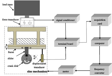
The displacement can be collected with a displacement transducer, and the acceleration is assumed to be the same for the frame and the base mass inside force transducer. The dynamic force could be obtained based on the determination of the inertia force as a known mass mounted on the force transducer [22].
2.1.1. Mathematical model
Force transducer can be described by the Voigt model, consisting of a spring mass system with stiffness and damping acting between the end mass and the base mass of the transducer [4]. When considering the influence of the coupling between the force transducer and the load mass , another spring mass system with stiffness and damping could be employed. Therefore, in this investigation, the schematic diagram illustrated in Fig. 2 can be used to represent the force transducer which is mounted in the calibration set-up.
Fig. 2Schematic diagram of a force transducer
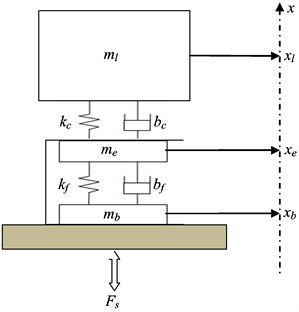
And the following differential equations could be established according to Fig. 2:
where , , are the vertical movements of the load mass, the end mass and the base mass respectively, is the acting force. Since the measured signals in this investigation are collected from the force transducer to be calibrated and the displacement transducer connected to the frame, our goal is to obtain the relationship between and . is proportional to the output signal of the force transducer to be calibrated, and can be collected with the displacement transducer.
To simplify system Eq. (3), take , , , and . In addition, the problem can be further considered in the Laplace space by introducing the complex variable to make the substitution , and the abbreviations and will be employed, too [7]. Thus system Eq. (3) can be expressed as following:
Take and transfer the algebraic equation system Eq. (4) into matrix formalism:
The solution of this system can be performed using Cramer’s rule [7]:
where:
To obtain the relationship between and , take as the target model:
When considering the influence of the coupling between the force transducer and the load mass, by substituting expressions of , , and into Eq. (7) we can obtain:
where:
In the case where the coupling of the load mass to the force transducer is very stiff, the transfer function Eq. (7) can be simplified using the limits and [7]:
where:
Since the system identification is finished in computer with application of advanced tools from Digital Signal Processing (DSP), we carry out transform with bilinear method for , where the constant realizes the transformation of the displacement into a force signal. And corresponding discrete transfer functions and for Eqs. (8) and (9) can be obtained as following:
where:
and is the sampling time.
where:
3. PSO based system identification
3.1. Schematic for system identification
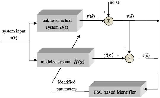
The main task of system identification is to search iteratively for the parameters of the modeled system such that the input-output relationship matches closely to that of the actual system [11]. The basic block diagram for system identification is shown in Fig. 3. System input is given to both the unknown system to be identified and the modeled system. The output mixed with a noise signal gives the final output to the actual system. On the other hand, the modeled system has an output of for the same input. The difference between the two output signals is used by the identifier to adjust the parameters [22]. Since traditional algorithms usually have difficulties in optimizing complex nonlinear systems, the identification of transfer Eqs. (10) and (11) will be finished with particle swarm optimization algorithm in this work.
Fig. 3Block diagram for PSO based system identification
3.2. PSO algorithm
Particle swarm optimization algorithm is initialized with a population of possible solutions called particles. Particles start flying from the initial positions through the search space with velocities exploring almost all optimal solutions. The velocity of each particle is dynamically adjusted according to its own flying experience and its companions’ flying experience, and the performance of each particle position is evaluated by a fitness function. During the flights, the best previous experience for each particle is stored in its memory and called the personal best (Pbest), and the best previous position among all particles is called the global best (Gbest) [10, 12, 22, 23].
Let be the position of the th particle, for Eq. (10) , and for Eq. (11) . Similarly, the velocity , the personal best and the global best are represented as and respectively. The particles are manipulated according to the following equations [10, 24]:
where acceleration coefficients are positive constant parameters with the constraint that control the maximum step size. Typically, , are both suggested to be 2.0. In [22] the authors also have studied the influence of acceleration coefficients , on PSO performance, and the results indicate that parameters and can get the tradeoff between identification accuracy and convergence speed. Therefore, and will be taken in this investigation. , are uniformly distributed random variables in the range [0, 1]. is the inertia weight and controls the impact of the previous velocity of the particle on its current one. In general, a bigger can guarantee the globally search ability, and avoid sinking into a local optimal solution. On the contrary, a smaller is good for local search, and can guarantee the convergence of the arithmetic. Thus, a self-adaptive adjusted strategy for inertia weight as follows can be taken [13]:
where is the current iteration generation, is the maximum iteration times, and are the minimum inertia weight and maximum inertia weight, respectively. The value of inertia weight in PSO is linearly decreased according to Eq. (14), and , are initial and final values for the inertia weight [23]. In this way, PSO tends to have more global search ability at the beginning of the run while having more local search ability near the end of the run [22]. and are generally taken in previous studies [14, 22].
In the system identification problem, PSO algorithm tries to minimize the error by adjusting the parameters of the modeled system. And mean square error (MSE) of time samples between the outputs of the actual system and the designed system as given by Eq. (15) is always considered as the fitness function [9, 11]. In mathematical statistics, mean square error is the mathematical expectation of differences between the estimated values and the truth values, and it is a convenient method to measure the average error:
where is the number of data points, is the output of the actual system, is the output of the modeled system with . The smaller the MSE value is, the higher accuracy of the modeled system is.
In general, the main problems of the PSO algorithm are slow convergence and premature convergence [25]. To deal with the problems, exponential transformation is introduced to the fitness function for helping quickly search the global optimal solution:
And with Eq. (16), the fitness function can be converted to a positive indicator in the range [0, 1].
3.3. Algorithm procedure
The implementation of PSO algorithm with exponential transformation (PSO+ algorithm) applied to system identification in this work is summarized as follows:
Step 1. Generate input-output data points to form the system to be identified.
Step 2. Set acceleration coefficients , , the maximum iteration times , and the scope of the inertial factors , that appear in Eqs. (12) and (14).
Step 3. Initialize the position and velocity for each particle. In this investigation, particle position corresponds to the parameters of transfer functions (10) and (11).
Step 4. Remember current particle position as Pbest of each particle. Find the particle with the best value of fitness function and remember its position as Gbest.
Step 5. Generate inertia weight and random numbers , in Eq. (12), and update the velocities and positions according to Eqs. (12) and (13).
Step 6. Evaluate fitness values and update Pbest and Gbest.
Step 7. Return to step 5 until the total number of iterations is achieved.
Step 8. Output the identified parameters namely Gbest and end the program.
4. Numerical simulations
4.1. Validation of PSO+ algorithm
For testing the performance of PSO+ algorithm, two benchmark functions listed in Table 1 which are similar to transfer functions Eqs. (10) and (11) are considered for the case studies. The inputs for the two studies are both . And the two cases are simulated with PSO and PSO+ algorithms in MATLAB with the following parameters: , , , population size, maximum position and maximum velocity are 150, 2 and 0.1 respectively. For case I, and the maximum generation is set to 1000. For case II, and the maximum generation is 2000. The transfer functions and their identification results are shown in Table 1. The outputs of actual systems and modeled systems for cases I and II are illustrated in Figs. 4 and 7 respectively. Figs. 5 and 6 are the curves of fitness functions for PSO and PSO+ in case I while Figs. 8 and 9 are those in case II.
From Figs. 4-9 and Table 1 we can see that, identification results of the two cases are in accordance with each other. Identification accuracies of PSO in the two cases are slightly higher than those of PSO+, but identification errors of PSO+ are very small too, since the MSE values listed in Table 1 are in the 10-17 order or less. From this point we know that, PSO+ algorithm is effective for system identification.
When comparing the convergence processes shown in Figs. 5-6 and Figs. 8-9, we can find that the convergence speed of PSO+ algorithm is obviously faster than that of PSO. For case I, PSO takes almost 880 iterations to converge to the global best while PSO+ takes less than 100 iterations. And for case II, PSO takes 1416 iterations to converge to the global best while PSO+ takes only 850 iterations. Consequently, we reach a conclusion that PSO+ algorithm can be used for system identification and it converges faster than conventional PSO.
Fig. 4Outputs for case I
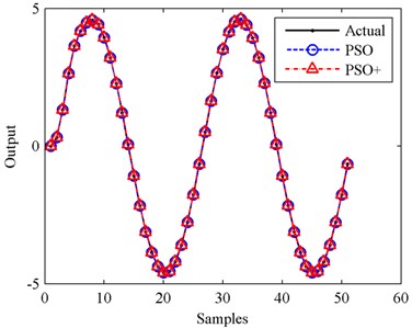
Fig. 5Fitness value of global best particle for PSO in case I
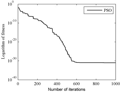
Fig. 6Fitness value of global best particle for PSO+ in case I
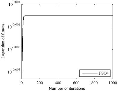
Fig. 7Outputs for case II
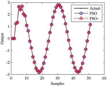
Fig. 8Fitness value of global best particle for PSO in case II
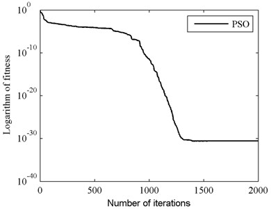
Fig. 9Fitness value of global best particle for PSO+ in case II
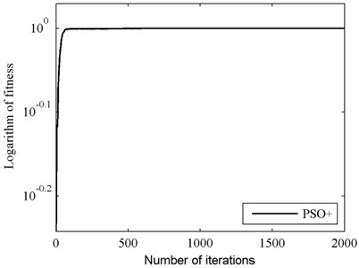
Table 1Identification results of benchmark systems
Case I | Case II | ||
Benchmark function | |||
Modeled systems | PSO | ||
PSO+ | |||
MSE | PSO | 1.0402e-31 | 2.5862e-31 |
PSO+ | 9.0450e-18 | 5.4054e-17 | |
4.2. Performance study of PSO+ in the presence of the additive noise
For studying the ability of PSO+ algorithm to operate in the presence of the additive noise, the benchmark function of case I listed in Table 1 is employed to finish another simulation study. The input for this study is still , and white noises of different signal to noise ratios (SNRs) are added to the output. The parameters of PSO+ algorithm is set as those in case I.
Fig. 10Output in the case of 50 dB SNR
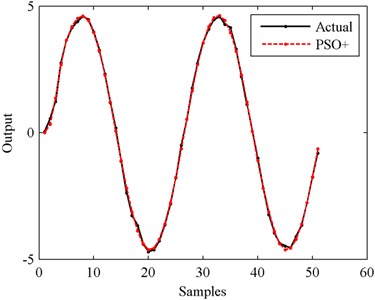
Fig. 11Output in the case of 40 dB SNR
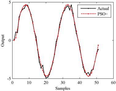
Fig. 12Output in the case of 30 dB SNR
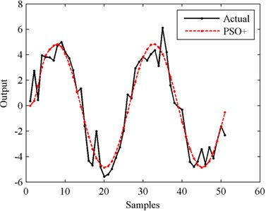
Fig. 13Output in the case of 20 dB SNR
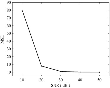
The outputs of actual systems and modeled systems are illustrated in Figs. 10-14 respectively. The MSE values are shown in Fig. 15.
From Figs. 10-14 we can see that, the higher the SNR is, the smoother the output curve is. And in this situation, the identification accuracy of PSO+ algorithm is higher, too. The relationship between identification accuracy and SNR is shown in Fig. 15. The MSE values in the cases of 10 dB-50 dB SNRs are 80.1880, 7.9021, 0.9229, 0.0921 and 0.0092 respectively. In all these situations, the outputs of the modeled systems can follow the changes of the actual outputs. But in order to obtain the higher identification accuracy, filtering process for the actual outputs is suggested to be finished before identifying with PSO+ algorithm.
Fig. 14Output in the case of 10 dB SNR
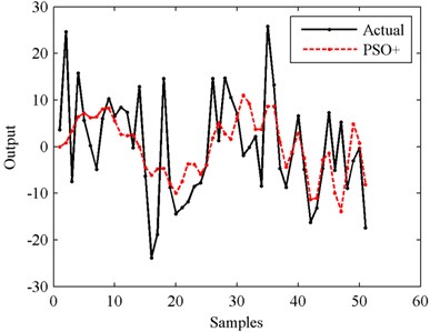
Fig. 15MSEs in the cases of different SNRs
5. Experiments and analysis
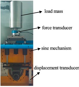
As described in Section 2, the experimental device shown in Fig. 16 is built. The transducer is calibrated with a top mass of 25.717 kg, which is connected to the transducer with a special mechanical adaption. The Minor KTC type displacement transducer is employed to measure the displacement of the frame. The signal from the force transducer is amplified with a SGA powered signal conditioner. An industrial computer with a PCI-1716L data acquisition card is used to record the two transducer signals through a PCLD-8710 terminal board [22].
Fig. 16The experimental device
5.1. Experiment I
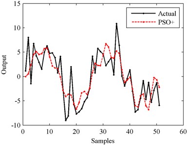
Firstly, the experiment is carried out with a force transducer of 5 kN. The sine mechanism is operating at a frequency of and the transducer signals are sampled at 20 kHz. After filtering and resampling, PSO+ algorithm is employed to identify the simplified function Eq. (11) (Case III) and function Eq. (10) (Case IV). 200 input-output data points are taken for system identification and another 400 data points are taken for testing. The parameters of PSO+ algorithm are set as follows: , , , population size and maximum position are 200 and 100 respectively. When identifying the simplified function Eq. (11), Recursive Least Squares (RLS) method is also used to do the identification besides the PSO+ algorithm. Alternative form of function Eq. (11) for RLS identification is shown below:
where:
Fig. 17 shows the identification errors of RLS and PSO+ for cases III and IV, and the convergence processes of fitness values for PSO+ algorithm are illustrated in Fig. 18. Testing results of the identified models for cases III and IV are shown in Fig. 19, and Fig. 20 shows the testing errors of the identified models with PSO+ algorithm. And for the empirical analysis of the testing results, MSE is employed as the accuracy evaluation standard which is shown in Table 2.
Fig. 17Identification errors for cases III and IV
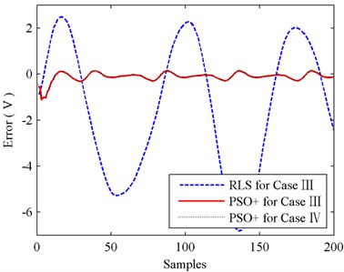
Fig. 18Fitness values of PSO+ for cases III and IV
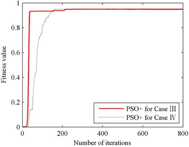
Fig. 19Testing results for cases III and IV
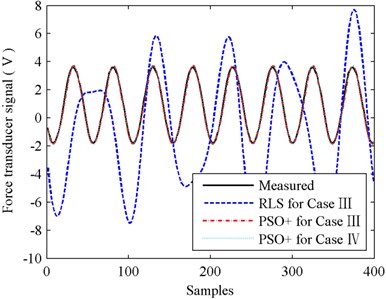
Fig. 20Testing errors of PSO+ for cases III and IV
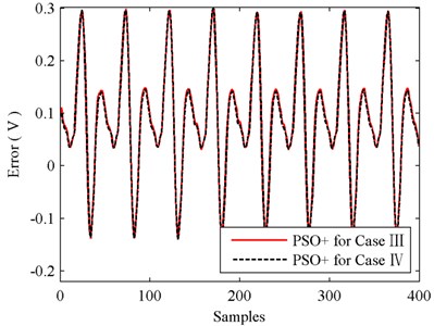
Table 2Testing results of experiment I
RLS for case III | PSO+ for case III | PSO+ for case IV | |
Testing MSE | 19.7667 | 0.0191 | 0.0186 |
The results shown in Figs. 17 and 19 indicate that, RLS is not suitable for the identification of function Eq. (11) since big errors exist in the processes of identifying and testing. The testing MSE values shown in Table 2 also tell this, as MSE of RLS is more than 1000 times bigger than MSE of PSO+. So, when compared with RLS, the identification performance of PSO+ for case III is encouraging.
When comparing the results of PSO+ for cases III and IV shown in Figs. 19-20 and Table 2, we can find that simplification between functions Eqs. (10) and (11) almost has no influence on identification accuracy. The testing MSE values of PSO+ for case III and IV are 0.0191 and 0.0186 respectively, identification accuracy in case IV is slightly better than that in case III. Nevertheless, in Fig. 18, we can see that the convergence speed of PSO+ for case III is faster than that for case IV. Therefore, by comprehensively considering the identification accuracy and convergence speed, we reach a conclusion that the simplification between functions Eq. (10) and (11) is feasible. And with the identified parameters obtained in case III we can calculate out the stiffness and damping of the force transducer conveniently. In this experiment, the stiffness and damping of the 5 kN force transducer are 0.291×10⁸ Nm-1 and 17136 Nsm-1 respectively.
5.2. Experiment II
For investigating the generality of this identification method, another force transducer of 12.5 kN is taken to carry out a same experiment. The parameters of PSO+ algorithm is set as those in experiment I. The identifications of 12.5 kN transducer for function Eq. (11) and function Eq. (10) are denoted as case V and case VI respectively. The identification results are shown in Figs. 21-24 and Table 3.
Fig. 21Identification errors for cases V and VI
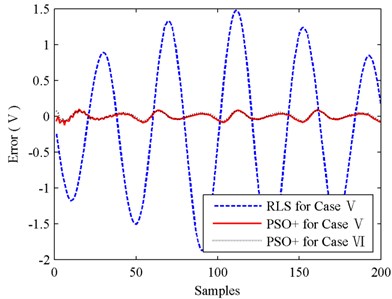
Fig. 22Fitness values of PSO+ for cases V and VI
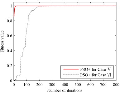
Fig. 23Testing results for cases V and VI
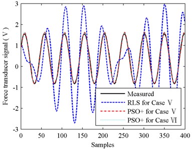
Fig. 24Testing errors of PSO+ for cases V and VI
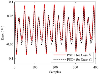
The results of experiment II are basically in accordance with those of experiment I. Identification error of RLS in Fig. 21 is still very big, and this leads to that the testing performance of RLS illustrated in Fig. 23 is not acceptable. Its MSE value is up to 0.9304 while MSE of PSO+ is only 0.0020. Then compare the identification performances of PSO+ for cases V and VI. As shown in Fig. 22, the convergence speed of PSO+ for case V is also faster than that for case VI obviously. The testing accuracies of PSO+ algorithm for cases V and VI are almost the same since MSE values of cases V and VI are 0.0020 and 0.0017 respectively. And with the identified parameters obtained in case V, the stiffness and damping of 12.5 kN force transducer are calculated as 0.246×10⁸ Nm-1 and 3032 Nsm-1 respectively.
Table 3Testing results of experiment II
RLS for case V | PSO+ for case V | PSO+ for case VI | |
Testing MSE | 0.9304 | 0.0020 | 0.0017 |
6. Conclusions
This paper represents a system set-up for dynamic calibrations of force transducers, and its mathematical model is derived in detail. For identifying the parameters of force transducers, PSO algorithm is introduced and a small modification is made to improve the convergence speed. Numerical simulations and experiments are carried out, and some conclusions are reached.
1) The sine mechanism described in this investigation is feasible for the dynamic calibration of force transducer.
2) The two experiments both indicate when PSO+ algorithm is employed to identify the simplified Eq. (11) and un-simplified Eq. (10), the identification accuracies are almost the same. Therefore, simplification between Eqs. (10) and (11) almost has no influence on system identification, and the mathematical approximation is reasonable.
3) PSO+ algorithm is effective for system identification, and with the aid of exponential transformation, the convergence speed of PSO+ is improved obviously.
References
-
Kumme Rolf Investigation of the comparison method for the dynamic calibration of force transducers. Measurement, Vol. 23, 1998, p. 239-2451.
-
Fujii Yusaku Toward dynamic force calibration. Measurement, Vol. 42, 2009, p. 1039-1044.
-
Fujii Yusaku A method for calibrating force transducers against oscillation force. Measurement Science and Technology, Vol. 14, 2003, p. 1259-1264.
-
Kumme R. Dynamic investigations of force transducers. Experimental Techniques, Vol. 17, 1993, p. 13-16.
-
Fujii Yusaku, Maru Koichi, Jin Tao, Yupapin Preecha P., Mitatha Somsak A method for evaluating dynamical friction in linear ball bearings. Sensors, Vol. 10, 2010, p. 10069-10080.
-
Zhang Li, Kumme Rolf Investigation of interferometric methods for dynamic force measurement. Proceedings of 17th IMEKO World Congress, Dubrovnik, Croatia, 2003, p. 315-318.
-
Schlegel Ch, Kieckenap G., Glöckner B., Buß A., Kumme R. Traceable periodic force calibration. Metrologia, Vol. 49, 2012, p. 224-235.
-
Link Alfred, Glöckner Bernd, Schlegel Christian, Kumme Rolf, Elster Clemens System identification of force transducers for dynamic measurements. Proceedings of 19th IMEKO World Congress, Lisbon, Portugal, 2009, p. 205-2071.
-
Luitel Bipul, Venayagamoorthy Ganesh K. Particle swarm optimization with quantum infusion for system identification. Engineering Applications of Artificial Intelligence, Vol. 23, 2010, p. 635-649.
-
Li Nai-Jen, Wang Wen-June, Hsu Chen-Chien James, Chang Wei, Chou Hao-Gong, Chang Jun-Wei Enhanced particle swarm optimizer incorporating a weighted particle. Neurocomputing, Vol. 124, 2014, p. 218-227.
-
Upadhyay P., Kar R., Mandal D., Ghoshal S. P. Craziness based particle swarm optimization algorithm for IIR system identification problem. International Journal of Electronics and Communications, Vol. 68, 2014, p. 369-378.
-
Tungadio D. H., Numbi B. P., Siti M. W., Jimoh A. A. Particle swarm optimization for power system state estimation. Neurocomputing, Vol. 148, 2015, p. 175-180.
-
Chen Yongbing, Song Yexin, Chen Mianyun Parameters identification for ship motion model based on particle swarm optimization. Kybernetes, Vol. 39, 2010, p. 871-880.
-
Tang Yang, Wang Zidong, Fang Jian-an Parameters identification of unknown delayed genetic regulatory networks by a switching particle swarm optimization algorithm. Expert Systems with Applications, Vol. 38, 2011, p. 2523-2535.
-
Zhang Wei, Ma Di, Wei Jin-jun, Liang Hai-feng A parameter selection strategy for particle swarm optimization based on particle positions. Expert Systems with Applications, Vol. 41, 2014, p. 3576-3584.
-
Alfi Alireza, Fateh Mohammad-Mehdi Parameter identification based on a modified PSO applied to suspension system. Journal of Software Engineering and Applications, Vol. 3, 2010, p. 221-229.
-
Nafar M., Gharehpetian G. B., Niknam T. Improvement of estimation of surge arrester parameters by using modified particle swarm optimization. Energy, Vol. 36, 2011, p. 4848-4854.
-
Yu Yu-zhen, Ren Xin-yi, Du Feng-shan, Shi Jun-jie Application of improved PSO algorithm in hydraulic pressing system identification. Journal of Iron and Steel Research, International, Vol. 19, 2012, p. 29-35.
-
Wu Zhitian, Wu Yuanxin, Hu Xiaoping, Wu Meiping Calibration of three-axis magnetometer using stretching particle swarm optimization algorithm. IEEE Transactions on Instrumentation and Measurement, Vol. 62, 2013, p. 281-292.
-
Andre Felipe Oliveira de Azevedo Dantas, Andre Laurindo Maitelli, Leandro Luttiane da Silva Linhares, Fabio Meneghetti Ugulino de Araujo A modified matricial PSO algorithm applied to system identification with convergence analysis. Journal of Control, Automation and Electrical Systems, Vol. 26, 2015, p. 149-158.
-
Xia Xin, Zhou Jianzhong, Xiao Jian, Xiao Han A novel identification method of Volterra series in rotor-bearing system for fault diagnosis. Mechanical Systems and Signal Processing, Vols. 66-67, 2016, p. 557-567.
-
Lu Jianshan, Xie Weidong, Zhou Hongbo Combined fitness function based particle swarm optimization algorithm for system identification. Computers and Industrial Engineering, Vol. 95, 2016, p. 122-134.
-
Marion Romain, Scorretti Riccardo, Siauve Nicolas, Raulet Marie-Ange, Krähenbühl Laurent Identification of Jiles-Atherton model parameters using particle swarm optimization. IEEE Transactions on Magnetics, Vol. 44, 2008, p. 894-897.
-
Al-Duwaish Hussain N. Identification of Hammerstein models with known nonlinearity structure using particle swarm optimization. Arabian Journal for Science and Engineering, Vol. 36, 2011, p. 1269-1276.
-
Galewski Marek A. Modal parameters identification with particle swarm optimization. Key Engineering Materials, Vol. 597, 2014, p. 119-124.
About this article

This project is supported by National Natural Science Foundation of China (Grant No. 51405437), the Key Laboratory of Intelligent Perception and Systems for High-Dimensional Information (Nanjing University of Science and Technology), Ministry of Education (No. JYB201609).
