Abstract
Operational modal analysis (OMA) has been utilized to extract structural dynamic characteristics by only using the output responses. In many cases of OMA, the problem of harmonic components, which is caused by periodic excitation components to the structure, may occur, and may lead to erroneous modal identification. In this paper, an optimized harmonic indicator function named the enhanced spectral kurtosis (ESK) is proposed to improve the effectiveness of the harmonic components detection. Moreover, a new algorithm based on virtual excitation assumption is presented to remove the harmonic components in modal parameters estimation. Finally, the quality of the proposed method is compared with that of the conventional method using a numerical simulation and a practical experiment.
1. Introduction
During the last decade, the modal analysis becomes a key technology in structural dynamics behavior study [1, 2]. Operational modal analysis (OMA) is a technology for the identification of the linear structural modal parameters by using only the output responses [3, 4]. It is used to derive an experimental dynamics model from vibration measurements on a structure in operational conditions. In many operational cases, it is impossible to measure the excitation force, and the structural responses are the only information that can be collected for the system identification algorithms. A new method based on the transmissibility function is proposed to process the parameters in OMA with unrestricted types load [5, 6], but it needs twice tests with different loads and may generate fake resonance peaks. Therefore, in the OMA, the system is generally assumed to be excited by a broadband random signal [7, 8]. However, in many applications, the presence of periodic excitation in the random loads is unavoidable. The periodic forces generated by unbalanced masses of rotating parts or aerodynamic or electric actuators, may cause harmonic components in the responses [9]. These harmonic components will cause uncertainty in extraction of modal parameters [10], and need to be detected and removed before modal identification.
A direct approach for processing the harmonic components in outputs is to take them as zero-damping modes. In practice, this method would not be effective when the structural modes have very low damping, or the harmonic frequencies are very close to the structural modal frequencies [11]. A method based on random decrement is proposed for distinguishing the harmonic frequencies from the natural frequencies [12, 13]. It argues that the harmonic components are un-attenuated. The harmonic components, in other words, are also assumed to be zero-damping modes in this method. Another method based on the probability density function (PDF) of the output for distinguishing a harmonic response from narrowband stochastic responses is widely used [9, 14, 15]. This method, however, is effective when the harmonic frequencies are well separated from the structural frequencies, since it would imply that temporal filter must be used. Furthermore, it will require tedious calculations and be restricted by bandwidth of the filter. A kurtosis-based method was initially proposed in time domain for distinguishing the random and period signals [16-18], and processed in a way similar to the PDF method mentioned above. In order to avoid tedious data calculation, the spectral kurtosis (SK) of a signal is defined as the kurtosis of its frequency component, and has been applied to harmonic components detection in the OMA [19-21]. Another advantage of this method is that the information of each frequency component can be indicated promptly in the frequency band of interest. However, the method is not perfect, since only one channel signal can be dealt with at a time. It brings a time-consuming problem and may lead to a failure of detection.
In order to improve the quality and efficiency of the harmonic components detection, an enhanced spectral kurtosis (ESK) based on the enhanced PSD function is proposed in this paper. Unlike the original SK method, the ESK calculation utilizes all multiple-channel signals at each resonance frequency of interest. Moreover, due to the application of a PSD enhancement technique, the band-pass filter is not required any more. Starting from the enhanced PSD obtained from the frequency spatial domain decomposition (FSDD) [22, 23], the ESK algorithm is derived in detail. Then, a new method named the virtual excitation technique (VET) is presented for the removal of harmonic components even when they are close to the natural frequencies. By using multiple input & multiple output (MIMO) model and virtual excitation assumption after detection of the harmonic frequencies, the responses which do not contain the harmonic components are obtained, and the structural model parameters are identified with these responses by the FSDD method. The result from the proposed method is also compared with that from the previous method by a numerical simulation. Finally, an application of the proposed method to detect and remove the harmonic component of a GARTEUR (Group of Aeronautical Research and Technology in EURope) aircraft model is presented to demonstrate its procedures and credibility.
2. Theory background
2.1. Detailed ESK description
Let be a discrete random signal, and its Discrete Fourier Transform (DFT), the original SK can be defined [19] as:
where denotes the operator of expectation and represents the modulus operator. In practice, the discrete sequence is divided into un-overlapped blocks to obtain an unbiased estimator of the SK by using the -statistics:
where the variables is a DFT of the th block. According to the statistical characteristic [19], the SK of a random process equals to zero. By contrast, the SK of a harmonic process always equals to –1 at the harmonic frequency. Supposing be mixed with a harmonic signal, the SK can be comprehensively described as:
where, is the harmonic frequency. Consequently, the harmonic components will be detected by computing the value of SK at each spectral line.
Assume that there are channels of output responses:
where superscript denotes the transposition. By applying the modal theory, the output responses in the physical space can be transformed into a modal subspace:
where is the mode shape matrix, and are the measured responses in modal and physical coordinates, respectively. The superscript denotes the Hermitian transposition. Therefore, the th single degree of freedom (SDOF) response can be derived as:
Then, the th SDOF response PSD can be computed as:
It is noticed that Eq. (8) has the same form with the enhanced PSD proposed in the FSDD technique for the OMA [22]. By inserting Eq. (7) into Eq. (2), the ESK for the th resonance peak can be defined as:
According to the Eq. (6), the statistics characters of the th SDOF response can be thought as stationary. Therefore, the ESK of a mixed-signal can also be derived as:
To sum up, the original SK calculation can only deal with one of multiple-channel signals at a time, and to ensure that the detection of harmonic components is not skipped, the SK of each (1, 2,…, ) should be calculated by using Eq. (2). The calculation becomes complicated if is a large number, which is common in the OMA. By contrast, the ESK is as an optimized method for multiple-channel signal processing.
Supposing that the th of ESK is close to zero, the th modal parameter can be extracted by using the enhanced PSD directly. The component, however, should be removed first in the case where its value of ESK is close to –1, particularly when it is close to a structural mode.
2.2. VET algorithm
The unknown mixed signal can be considered as the linear superposition of a random signal and a harmonic signal:
where is a random signal and is a harmonic signal. In the frequency domain, the random signal can be assumed as the product of a virtual white noise (constant spectrum) and a function of coefficient . Similarly, the harmonic signal can be assumed as the product of a virtual harmonic signal and a constant coefficient . The DFT of the mixed signal can be expressed with the virtual excitations as:
Indeed, the spectrum of the random input is not always flat in practice, but can be generally considered as constant spectrum in a narrow band [23]. The MIMO model can be written at each frequency in the narrow band as:
where is the frequency response function (FRF) matrix of the system, and is a constant coefficient. Using the Least Squares algorithm, the proportional virtual responses of this system can be obtained as:
where the superscript + denotes pseudo inversion, and Therefore, the response by the virtual excitations can be obtained as:
It is obvious that the does not contain the harmonic modes any more, which means the harmonic components are removed successfully.
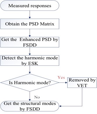
In order to improve the understandability of the method, a flow chart is given as follows:
Fig. 1Flow chart of identification based on ESK and VET
3. Numerical case
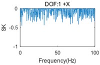
A two-storey building structure with six DOFs (regarding two floors as two lumped masses, each lumped mass has two translational DOFs and a rotational DOF), shown in Fig. 2, is used to validate the proposed algorithm. The simulation technique based on the FRF modes is employed to generate six responses with five uncorrelated random noise signals and a mixed signal with a periodic frequency at 33.4 Hz in the -direction. The simulated time domain responses have a length of 204, 800 points, with a sample frequency of 256 Hz. The PSD matrix of responses will be computed by the Welch method, using Hanning windowing and resolution of 0.2 Hz. Then, the mode indicator function (MIF) curves can be computed by singular value decomposition (SVD) in 0-100 Hz, as shown in Fig. 3. The original SK method is used to detect a harmonic component and the results are shown in Fig. 4.
Fig. 2Two-storey building model
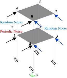
Fig. 3Mode indicator curves of two-storey building
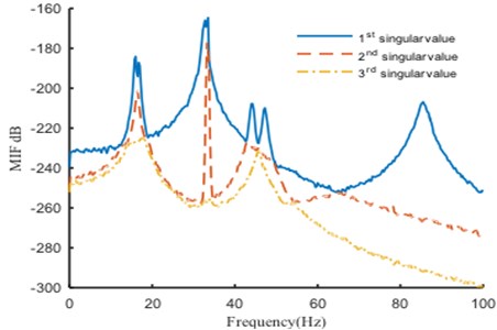
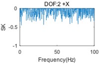
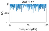
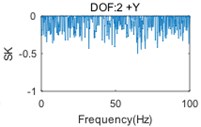
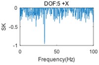
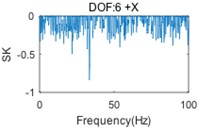
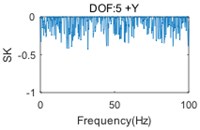
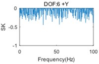
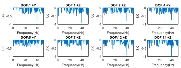
Fig. 4SK curves of responses (two-storey building)
a)
b)
c)
d)
e)
f)
g)
h)
In Fig. 3, the first (solid) curve, second (dash) curve and third (dotted) curve consist of the 1st, 2nd and 3rd singular value at each spectral line, respectively. Six structural modes and a harmonic component (at the frequency of 33.4 Hz) are apparently indicted by the mode indicator curves. Moreover, the harmonic component is very close, actually only three spectral lines are far, to the 3rd natural frequency. Fig. 4 shows that the harmonic is not always indicated by SK of response at each DOF, since the harmonic component(s) may not, in general, be strongly contained in all measured responses. Therefore, the SK of all responses should be calculated for a good harmonic detection. Moreover, although the harmonic is indicated in several SK curves, like Fig. 4(e) and Fig. 4(f), the SK values at the harmonic frequency are not exact –1 as expected. Since the frequency band is too narrow to separate harmonic frequency from nearby structural frequency by band-pass filtering, the computational accuracy is influenced.
The th (1, 2,…, 7) ESK curve is computed by Eq. (6) and Eq. (8) after picking the corresponding peak in the MIF curve, as shown in Fig. 5. It is clearly observed that the 4th (harmonic component) ESK value at 33.4 Hz is very close to –1, which means that the harmonic component has been indicated successfully. In contrast with the SK method, the ESK method is more reliable to detect the harmonic components, because all of the measured responses are completely considered by the calculation of ESK from the enhanced PSD.
Fig. 5ESK curves at each peak (two-storey building)
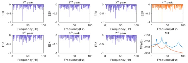
Furthermore, Fig. 5 shows that the harmonic frequency is also indicated by other ESK curves (such as the first and third one), since the harmonic component is not always completely decoupled from the structural modes. As a result, the enhanced PSD of a structural mode may contain the harmonic component as well. Accordingly, the harmonic component should be removed to avoid the errors during the identification of modal parameters, especially when the harmonic frequency is close to a modal frequency. The virtual harmonic input signal can be assumed as: and the random input signal is assumed as virtual white noise . According to the Eq. (12) and Eq. (13), the third enhanced power spectral density of virtual response is proportional to that of the real response except at harmonic frequencies in a narrow band, as shown in Fig. 6(a). For comparison, the constant of proportionality is normalized, as shown in Fig. 6(b).
Fig. 6Enhanced PSD curve in narrow band before and after harmonic component removal
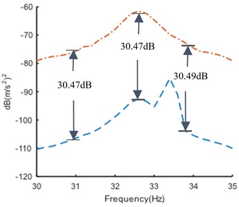
a)
b)
It should be noted that they do not match completely (shown in Fig. 6(b)), because the assumed excitation is uncorrelated with the real excitation (see Eq. (10)), which means the assumed excitation is indeed noise. Fortunately, the noise level is acceptable to identify the modal parameters by FSDD method. The modal frequencies and damping ratios identified before and after harmonic components removal are shown in Table 1 and Table 2, respectively.
Table 1Modal frequencies before and after harmonic component removal
Mode No. | Mode 1 | Mode 2 | Mode 3 | Harmonic | Mode 4 | Mode 5 | Mode 6 |
Harmonic contained (Hz) | 15.94 | 16.82 | 33.10 | 33.40 | 44.12 | 47.18 | 85.46 |
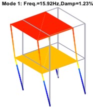
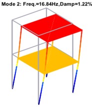
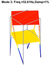
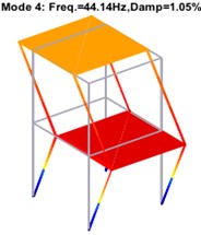
Harmonic removed (Hz) | 15.92 | 16.84 | 32.61 | – | 44.14 | 47.17 | 85.46 |
Theoretical (Hz) | 15.93 | 16.86 | 32.65 | – | 44.18 | 47.13 | 85.47 |
As shown in Table 1 and Table 2, the relative error of the 3rd modal damming ratio is up to 24 % before the harmonic removal, but it is corrected after the harmonic removal. The modal assurance criterion (MAC) is introduced to check the orthogonality between the theoretical and identified mode shapes, as shown in Fig. 7. The mode shapes identified after harmonic component removal are shown in Fig. 8.
It is seen in Fig. 7 that the orthogonality of the mode shapes is greatly improved after the harmonic removal. The analytical results indicate that the removal of harmonic components is an efficient way to adjust the structural modes. It also proves that the proposed method is an effective tool to remove the harmonic components in OMA.
Table 2Damping ratios before and after harmonic component removal
Mode No. | Mode 1 | Mode 2 | Mode 3 | Harmonic | Mode 4 | Mode 5 | Mode 6 |
Harmonic contained (%) | 1.28 | 1.22 | 1.24 | 0.15 | 1.00 | 1.03 | 1.54 |
Harmonic removed (%) | 1.23 | 1.22 | 1.00 | – | 1.05 | 1.05 | 1.52 |
Theoretical (%) | 1.25 | 1.21 | 1.00 | – | 1.05 | 1.08 | 1.53 |
Fig. 7Modal assurance criterion (MAC)
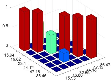
a) MAC before harmonic components removal
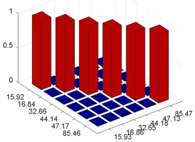
b) MAC after harmonic components removal
Fig. 8Structural modes of two-storey building after harmonic component removal
4. Experimental case
The technique discussed above is applied to the GARTEUR aircraft model in the laboratory. Two shakers are fixed in two directions respectively, as shown in Fig. 9. A random noise of 0-128 Hz is applied on the bottom of the structure by one shaker, and a harmonic load of 39.15 Hz is applied on the middle of the structure by another shaker. The experiment is performed with 102, 400 points at a sampling frequency of 128 Hz. The acceleration responses of thirty-four DOFs are obtained in time domain, as shown in Fig. 10. The PSD matrix of responses is computed by the Welch method, with Hanning window applied. The frequency resolution is 0.08 Hz. The FSDD mode indicator curves of response signals, with nine resonance peaks indicated, are showed in Fig. 10. The first peak is the rigid body mode caused by rubber cord suspension, and the fifth peak is the harmonic component which is very close to the fourth structural mode. The original SKs of the thirty-four measured responses are computed to detect the harmonic component, and part of them is shown in Fig. 11.
Fig. 9Experimental scene
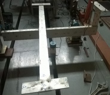
Fig. 10Typical time response (top) and mode indicator curves (bottom) of GARTEUR
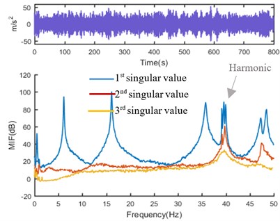
Fig. 11SK curves of responses (GARTEUR)
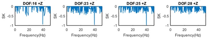
The SK curves in Fig. 11 are not always effective enough to indicate the harmonic component, since the computational accuracy is affected by the band-pass filtering. Therefore, the SKs of all measured responses should be calculated and examined to make sure that there are no missing harmonics in practice. By comparison, there are only nine ESKs that need to be computed, and the results are shown in Fig. 12. It is observed that the harmonic is clearly indicated by the 5th ESK value at 39.15 Hz. It is also noticed that the computation of the SKs takes about 12.68 seconds, while the computation of the ESKs (including SVD) needs only about 3.03 seconds on the same computing platform. It turns out that the ESK method is more reliable and efficient to detect the harmonic components than the original SK method.
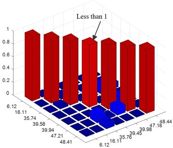
Fig. 12ESK curves at each peak (GARTEUR)
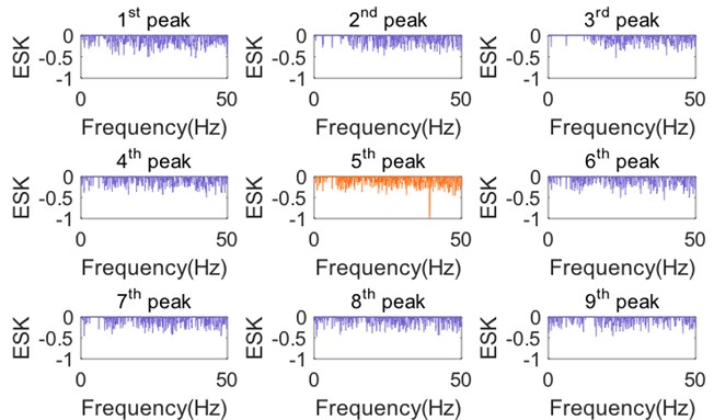
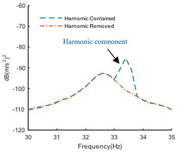
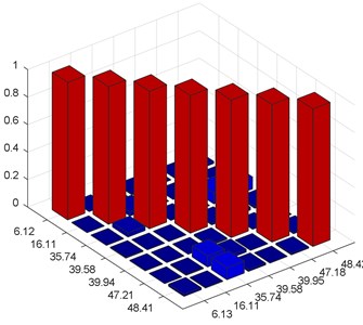
The harmonic component may affect the modal parameters identified by FSDD, since it is close to the 5th mode (6th peak) and 6th mode (7th peak) and cannot be decoupled in the enhanced PSD. Therefore, the harmonic component, which has been detected, should be removed by using the VET. The comparison of the enhanced PSD before and after harmonic component removal is shown in Fig. 13.
Fig. 13Enhanced PSD of 5th and 6th mode enhanced PSD curves in narrow band before and after harmonic component removal
As shown in Table 3 and Table 4, the relative error of the 4th and 5th modal damming ratios are up to 57.14 % and 50 %, respectively, before the harmonic removal, but they are modified after the harmonic removal. The MAC is used to check the orthogonality between the reference and identified mode shapes, as shown in Fig. 14.
Table 3Modal frequencies of GARTUER before and after harmonic components removal
Mode no. | Mode1 | Mode2 | Mode3 | Harmonic | Mode 4 | Mode 5 | Mode 6 | Mode 7 |
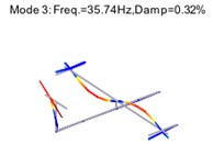
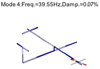
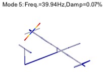
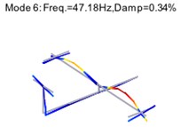
Harmonic contained (Hz) | 6.12 | 16.11 | 35.76 | 39.15 | 39.45 | 39.98 | 47.18 | 48.44 |
Harmonic removed (Hz) | 6.13 | 16.11 | 35.74 | – | 39.58 | 39.95 | 47.18 | 48.42 |
Only random excitation (Hz) | 6.12 | 16.11 | 35.74 | – | 39.58 | 39.94 | 47.21 | 48.41 |
Table 4Damping ratios of GARTUER before and after harmonic components removal
Mode No. | Mode1 | Mode2 | Mode3 | Harmonic | Mode 4 | Mode 5 | Mode 6 | Mode 7 |
Harmonic contained (%) | 0.20 | 0.18 | 0.33 | 0.06 | 0.11 | 0.10 | 0.28 | 0.22 |
Harmonic removed (%) | 0.13 | 0.17 | 0.32 | – | 0.08 | 0.07 | 0.33 | 0.22 |
Only random excitation (%) | 0.13 | 0.15 | 0.31 | – | 0.07 | 0.05 | 0.30 | 0.18 |
Fig. 14Modal assurance criterion (MAC)
a) MAC before harmonic components removal
b) MAC after harmonic components removal
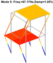
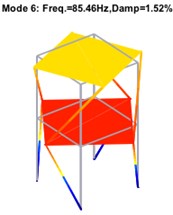
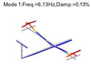
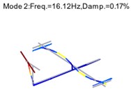
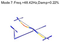
The improvement of the orthogonality (note the MAC value of the 4th mode) can also be observed after the harmonic removal. The experimental results prove that the proposed method is an effective tool to remove the harmonic components in the OMA. Then, the structural mode shapes in 0-50 Hz are obtained after harmonic component removal as shown in Fig. 15.
Fig. 15Mode shapes of GARTUER after harmonic components removal
5. Conclusions
Harmonic components make a difference in the dynamical response of many structural or mechanical systems which are excited by periodic loads. It is a challenge for many OMA techniques to detect and remove the harmonic components.
The ESK method is proposed in this paper to optimize the process and result of the harmonic component detection. It takes all multiple-channel signals at each resonance frequency into account by the enhanced PSD function. Less computation than the original SK method is asked, because the number of measured DOFs is generally larger than the number of modes in the OMA. It can also improve the accuracy of computation and avoids the risk of the harmonic component(s) absence by computing the enhanced mode.
The VET method is presented in this paper for the removal of harmonic components. By assuming the Multiple Input Multiple Output (MIMO) model and virtual noise excitation, the responses without harmonic components are obtained by the Least Squares (LS) algorithm. Then the accuracy of identified modal parameters can be greatly improved for the modes highly coupled by the harmonic component.
The results of the simulation and experiment demonstrate that the presented harmonic detection and removal methods are efficient and credible.
References
-
Yayli M. O. On the axial vibration of carbon nanotubes with different boundary conditions. Micro and Nano Letters, Vol. 9, Issue 11, 2014, p. 807-811.
-
Yayli M. O. Free vibration behavior of gradient elastic beam with varying cross section. Shock and Vibration, Vol. 2014, 2014, p. 1-11.
-
Ventura C. E., Horyna T. Structural assessment by modal analysis in Western Canada. Proceedings of 15th International Modal Analysis Conference, Orlando, Florida: International Society for optical Engineering, 1997, p. 234-239.
-
Araújo I. G., Laier J. E. Operational modal analysis using SVD of power spectral density transmissibility matrices. Mechanical Systems and Signal Processing, Vol. 46, Issue 1, 2014, p. 129-145.
-
Liu P. K., Shao X. J., Zhou F. M., et al. A study on the application of the operating modal analysis method in selfpropelled gun development. Journal of Vibroengineering, Vol. 18, Issue 3, 2016, p. 1683-1691.
-
Devriendt C., Sitter G. D., Vanlanduit S., et al. Operational modal analysis in the presence of harmonic excitations by the use of transmissibility measurements. Mechanical Systems and Signal Processing, Vol. 23, Issue 3, 2009, p. 621-635.
-
Brincker R. Some elements of operational modal analysis. Shock and Vibration, Vol. 2014, 2014, p. 1-11.
-
Reynders E., Houbrechts J., Roeck G. D. Fully automated (operational) modal analysis. Mechanical Systems and Signal Processing, Vol. 29, Issue 5, 2012, p. 228-250.
-
Brincker R., Kirkegaard P. H. Special issue: operational modal analysis. Mechanical Systems and Signal Processing, Vol. 24, Issue 5, 2010, p. 1209-1212.
-
Rainieri C., Fabbrocino G., Manfredi G., et al. Robust output-only modal identification and monitoring of buildings in the presence of dynamic interactions for rapid post-earthquake emergency management. Engineering Structures, Vol. 34, 2012, p. 436-446.
-
Mohanty P., Rixen D. J. Operational modal analysis in the presence of harmonic excitation. Journal of Sound and Vibration, Vol. 270, Issues 1-2, 2004, p. 93-109.
-
Modak S. V. Separation of structural modes and harmonic frequencies in operational modal analysis using random decrement. Mechanical Systems and Signal Processing, Vol. 41, Issues 1-2, 2013, p. 366-379.
-
Modak S. V., Rawal C., Kundra T. K. Harmonics elimination algorithm for operational modal analysis using random decrement technique. Mechanical Systems and Signal Processing, Vol. 24, Issue 4, 2010, p. 922-944.
-
Brincker R., Andersen P. An indicator for separation of structural and harmonic modes in output-only modal testing. Proceedings of the European COST F3 Conference on System Identification and Structural Health Monitoring, Universidad Politécnica de Madrid, Spain, 2002, p. 265-272.
-
Modak S. V. Influence of a harmonic in the response on randomdec signature. Mechanical Systems and Signal Processing, Vol. 25, Issue 7, 2011, p. 2673-2682.
-
Dion J. L., Chevallier G., Festjens H. Tracking and removing modulated sinusoidal components: a solution based on the kurtosis and the extended Kalman filter. Mechanical Systems and Signal Processing, Vol. 38, Issue 2, 2013, p. 428-439.
-
Agneni A., Coppotelli G., Grappasonni G. A method for the harmonic removal in operational modal analysis of rotating blades. Mechanical Systems and Signal Processing, Vol. 27, 2012, p. 604-618.
-
Andersen P., Brincker R. Using EFDD as a robust technique for deterministic excitation in operational modal analysis. Proceedings of the 2nd International Operational Modal Analysis Conference, Copenhagen, Denmark, 2007, p. 193-200.
-
Vrabie V., Granjon P., Servière C. Spectral kurtosis: from definition to application. Proceedings of the 6th IEEE NSPI Grado-Trieste, Italy, 2003.
-
Antoni J. The spectral kurtosis: a useful tool for characterising non-stationary signals. Mechanical Systems and Signal Processing, Vol. 20, Issue 2, 2006, p. 282-307.
-
Dion J. L., Tawfiq I., Chevallier G. Harmonic component detection: optimized spectral kurtosis for operational modal analysis. Mechanical Systems and Signal Processing, Vol. 26, Issue 1, 2012, p. 24-33.
-
Wang T., Celik O., Catbas F. N., et al. A frequency and spatial domain decomposition method for operational strain modal analysis and its application. Engineering Structures, Vol. 114, Issue 1, 2016, p. 104-112.
-
Zhang L. M., Wang T., Tamura Y. A frequency-spatial domain decomposition (FSDD) method for operational modal analysis. Mechanical Systems and Signal Processing, Vol. 24, Issue 5, 2010, p. 1227-1239.
Cited by
About this article

This research was supported by the Aeronautical Science Foundation of China (Grant No. 20161352011).
