Abstract
A rotor-to-stator coupled system usually exhibits complicated dynamic behaviors due to its nonlinear nature. Moreover, the inherent uncertainty (aleatory uncertainty) and many undetermined factors either brought by manufacturing process or due to the lack of knowledge (epistemic uncertainty) make the analysis of system response a challenging task. Existing studies on rotor uncertainties are mostly focused on the stochastic variables, yet pay less attention to other forms of uncertain variables such as intervals. However, some physical parameters (e.g. friction coefficient) can be hardly assigned one specific probability distribution and often available in interval forms. To deal with this, the concept of likelihood is extended from classical discrete point value to interval variable in the presence of mixed uncertainties. A likelihood-based approach is carried out for the mixed uncertainties representation and quantification. In addition, a new single loop sampling algorithm is developed to reduce the computation cost. This framework could be applied in the field of industry manufacturing and mounting, especially take effect in risk assessment and product maintaining. A series of numerical cases are demonstrated for validation and comparison.
1. Introduction
Motivated by the requirement to enhance the efficiency in engineering, the speed of rotating machinery is continuously increasing while the gap between the rotor and stator is significantly reduced. Affected by various uncertain factors, the rotor/stator rubbing is not rare in practical engineering. Unexpected rub induced by instability may lead to catastrophic consequence.
In the deterministic research field, a large amount of work has been done to better understand the rub-related phenomenon and get deep insights into its physical nature. Black [1] first discovered the existence condition of the synchronous full annular rub solution in early 1680s. Later Muszynska [2, 3] reported many possible responses of rotor/stator system. Through the numerical and experimental investigations, many typical contact responses as well as nonlinear dynamic behaviors have been captured, for instance, the jump phenomenon and the synchronous full annular rubs [4, 5], the partial rubs in sub- and super-synchronous whirl [6-8], the partial rubs in quasi-periodic whirl [9, 10], the chaotic motion [11-13] as well as dry whip [14-17]. In the last decade, Jiang etc. [18, 19] discussed the physical mechanism of dry whip and analytically derived the onset/existence conditions for a modified Jeffcott rotor.
However, the parameter uncertainty is inherent in most practical engineering and its effect on system response should not be overlooked. This problem has been realized in recent years and addressed in a series of publications [20-23]. These research works have made great contributions to the field of design and assessment of rotor/stator system considering parameter uncertainty. However, most of these monographs are concentrating on the parameters stochastic nature. From the perspective of uncertainty theory, the uncertainty that they are dealing with is pure aleatory uncertainty. The global response of a rotor/stator system under mixed uncertainty is still unclear. This issue is challenging in dynamic analysis or reliability evaluation and has not been sufficiently addressed yet. To fill the research gap and establish a more generic framework, this article proposes a likelihood-based approach for uncertain dynamic analysis or reliability estimation. Limitations embedded in traditional methods have been eliminated by extenging the concept of likelihood from traditional sparse point data to interval information. A single loop sampling algorithm is developed to simplify the computing process.
This paper is organized as follows, the modified Jeffcott rotor/stator system and its corresponding governing equations are presented in section 2, along with the analyses of dynamics and stability under ideal circumstance (deterministic) in section 3. The basic principle and detailed algorithm of the proposed likelihood-based approach are illustrated in section 4. Several numerical cases are demonstrated for validation and comparison purpose in section 5. The benefits and possible experimental verification are discussed in section 6. Finally, some concluding remarks are drawn.
2. Mathematical model and motion equation
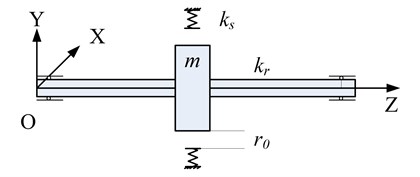
A modified Jeffcott rotor/stator system is taken into study shown as Fig. 1, which is comprised of an eccentric rotor and a rigidly fixed stator with elastic surface. The rotor consists of a massless shaft carrying a disk with mass mounted at the middle of the span. The disk mass center deflects its geometrical center with a distance , namely, the rotor has an eccentricity . This leads a mass imbalance when the rotor rotates at a speed . The stiffness of rotor shaft is denoted as and the stator is approximated modeled by radial springs with stiffness . There is an initial clearance between the rotor and stator.
Fig. 1a) Schematic diagram of the rotor/stator system, b) applied forces of rotor during whirling
a)
b)
The motion equation is given as:
where the damping ratio, Coulomb friction coefficient are denoted by and respectively. Eq. (1) can be rewritten in the non-dimensional form and formulated as:
where the non-dimensional variables are defined as:
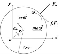
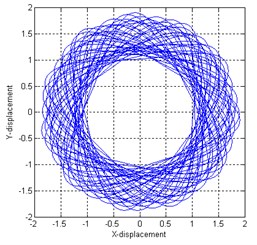
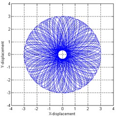
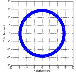
It is apparent that the motion equation is linear when the rotor is separate from the stator (i.e. 0). However, if the displacement of the rotor center exceeds initial clearance, the rotor would get in contact with the stator and the motion equation becomes nonlinear. This rotor/stator system has complicated dynamic behaviors with nonlinear characteristics. The various responses of the rotor/stator system (periodic full annular rub, quasi-periodic partial rub and dry whip, see in Fig. 2) with different given parameters will be discussed in the next section.
Fig. 2Rotor orbit for different parameters: a) full annular rub, b) partial rub, c) dry whip
a)
b)
c)
3. Deterministic system response and stability analysis
Since our goal is to better understand the responses of rotor/stator system considering uncertainty, it is necessary to study the dynamics behaviors under deterministic condition. There are multi-types of responses of the rotor/stator system which are governed by different motion equations depending on the input parameters. For instance, if the deflection of the rotor center is less than the gap between rotor and stator, the rotor is not in contact with stator and the motion equation becomes linear. When the rotor gets full contact with the stator, it is the full annular rub that has been observed in the experiment [17, 24, 25]. However, if the rotation speed continuous goes up, the rotor may lose its stability, the system response becomes quasi-periodic and the motion is partial rub. In other cases, the friction direction is changed due to the high rotation speed or crude contact surface, which leads to a backward whirl motion (dry whip). Relative research works could refer [14-16]. For mathematical convenience, the motion equation is rewritten in the vector form as:
where:
The steady-state periodic solution is in the form as , . Eq. (3) is linearized about the steady-state solution (, ) as:
where is a derivative operator and is the Jacobian matrix. If we use to represent a perturbation of the steady solution (, ), the stability of is able to reflect the stability of solution (, ). Hence, the stability of the corresponding solution of Eq. (4) could be utilized to determine stability of solutions in Eq. (3) and thus, the stability for both linear solution and nonlinear solution [5].
3.1. Deterministic boundary for linear solution
For the linear scenario, the rotor will not contact with the stator, namely, 0. Thus, the govern equation reduce to:
The steady-state periodic solution is presented in the form as . The amplitude and phase angle are given by:
However, this solution is only eligible when the amplitude is less than clearance . Let , the parameter equation for no rub periodic solution is derived as Eq. (7):
On the other hand, the associated characteristic equation for Jacobian matrix is expressed as:
By adopting the Routh-Hurwitz condition, it is found that the solution is always stable since . Thus, the two real roots and , which solved from Eq. (7), can be used to determine the stable boundary of no-rub motion.
3.2. Deterministic boundary for nonlinear solution
When the rotor get in contact with the stator, i.e. 1 the governing equation becomes nonlinear. For this scenario, the Jacobian matrix is time-dependent and is in following form:
To study the stability of one specific solution, corresponding transformation is taken as:
where:
thus, Eq. (11) is derived by substituting Eq. (10) into Eq. (4):
Define and the is solved as:
Now, the time-dependent component is separated from the Jacobian matrix and the time-independent matrix can be used to evaluate the stability of solution. The characteristic equation is written as:
where denotes the eigenvalues of and coefficients are determined as:
As these eigenvalues are related to the amplitude and should be first solved and substituted into Eq. (13). Then the Routh-Hurwitz criteria can be adopted to evaluate the stability of nonlinear solution. For more details, please refer [5]. However, since our goal is not only to judge the stability of one given solution but also to determine the safe region in the parameter space, the parameter boundary is analyzed from the bifurcation perspective.
3.2.1. Saddle-node bifurcation
Based on the saddle-node bifurcation theory, there should be one zero eigenvalue of the Jacobian matrix. By substituting 0 into characteristic equation, it leads to:
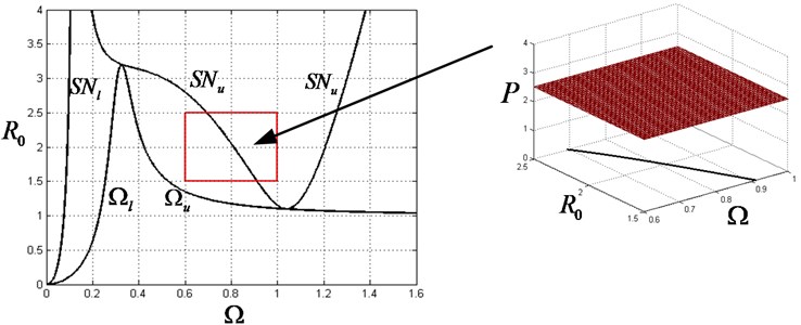
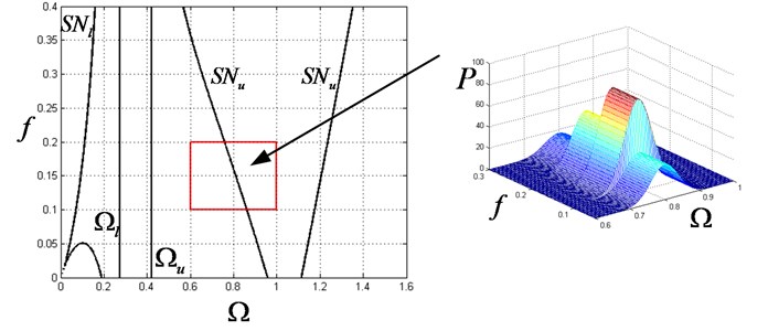
By eliminating the amplitude through symbolic calculation, a twelve-order polynomial of rotation speed is derived. With the aid of numerical simulation, saddle-node bifurcation boundaries can be solved and depicted on the parameter region.
3.2.2. Hopf bifurcation
According to the Hopf bifurcation theory, there should be one pair of conjugate purely imaginary eigenvalues (e.g. or ) for the Jacobian matrix. By substituting (or ) into the characteristic equation, Eq. (15) is derived as:
Eliminating , it leads to:
By Substituting - in Eq. (13) into Eq. (16) and after manipulation, Eq. (17) is derived as:
where the coefficient - is given as:
After eliminating , a twelve-order polynomial of rotation speed is also obtained and the boundary of Hopf bifurcation can be numerically solved.
4. Likelihood-based representation of epistemic uncertainty due to sparse point data and interval data
In previous section, the system response in ideal circumstance, i.e. the deterministic boundary in parameter region, has been studied. In this section, multi-source uncertain factors within the system are taken into account and a likelihood-based approach dealing with mixed uncertainty is developed.
4.1. Description of uncertainty
In practical engineering, many uncertain factors (e.g. physical uncertainty, model uncertainty) are induced either by biased experiential judgments or by lack of knowledge. To quantify them, an unified measurement need to be built. According to the recently developed uncertainty theory, the uncertainty can be mainly classified into two groups, i.e. aleatory uncertainty and epistemic uncertainty. This distinction for uncertainty has been recognized by the NNSA and emphasized in the NAS/NRC report about QMU (Quantification of Margins and Uncertainties). For the basis and rationale of uncertainty theorem, please refer relevant monographs or publications [26-32].
The aleatory uncertainty arises from an inherent randomness in the properties or behavior of the system under study. On the other hand, the epistemic uncertainty derives from a lack of knowledge about the appropriate value to use for a quantity that is assumed to have a fixed value in the context of a particular analysis [26]. The aleatory uncertainty is supposed to be irreducible and usually represented in the stochastic form. By contrast, the epistemic uncertainty can be reduced when new information becomes available, it is represented in more complicated forms as both probabilistic and non-probability variable may coexist. (e.g. interval or point data). In this paper, both aleatory and epistemic uncertainties are taken into consideration.
4.2. Construction to the likelihood of uncertain interval data
In this subsection, the concept of likelihood function is first reviewed and extended from classical sparse point data (deterministic) to interval information (uncertain), which serves the foundation of the likelihood-based approach.
Consider a stochastic variable follows one specific distribution (e.g. Normal) with a series of collected point data, its PDF (Probability Density Function) is denoted as where corresponds to the parameter set. The likelihood function is defined as the probability of a series of given data set conditioned on distribution parameter [30, 33, 34]. Theoretically speaking, the probability value for any single discrete point is zero for a continuous density function, the likelihood function is obtained by considering the probability of an infinitesimally small interval around based on mean value theorem as Eq. (18) for practical use in previous work [30, 33, 34]:
The parameter can be evaluated by maximizing the right hand side of Eq. (18). This estimation approach is popularly known and widely adopted as the maximum likelihood estimate (MLE).
Similar principle can be extended to bounded interval data, thus the expression for likelihood of the parameters for interval [, ] is:
where the corresponds to the CDF (Cumulative Density Function) of variable . For multiple input interval information, the combined likelihood function is expressed as:
It is the CDF rather than PDF that will be used in the likelihood calculation for interval data, compared with that for point data. This is the main difference between the construction of likelihood for conventional point data and interval data.
4.3. Representation of epistemic uncertainty with additional probabilistic information
Sometimes, additional probabilistic information is available for the uncertainty variable besides the given intervals and/or sparse point data. For instance, the rotor eccentricity may be given by a series of intervals based on expert judgments and some sparse point collected from the measurements of similar product in this case. On the other hand, from the physical background perspective, the uncertainty of eccentricity mainly arise from the error/deviation accumulated during the procedure of manufacturing, mounting, etc., which generally follows the normal distribution (statistics parameter is unknown).
For this scenario, if variable is supposed to follow one specific distribution, the combined likelihood function can be expressed as Eq. (21). Since the comprehensive likelihood is expressed as Eq. (21), the distribution of parameter can be derived utilizing the MLE. However, this calculation may be cumbersome because the cumulative density function of variable is not always in analytical form (e.g. the CDF of normal distribution). In this paper, instead of computing statistics parameter by maximizing the likelihood, a Bayesian-based approach is adopted to estimate the full likelihood. The idea that the entire likelihood function, rather than merely its maximizer, should be used for inference was emphasized by Barnard et al. [35]:
Assigning an appropriate prior distribution, the parameter is estimated as Eq. (22) by adopting Bayesian theory:
where denote the joint prior distribution of parameter vector , while is the estimated probability distribution of . is the combined likelihood function which has the same form as Eq. (21).
It should be noted that the parameter estimated in Bayesian method is a probability distribution, compared with a deterministic value by MLE method. Hence, a family of conditioned probability distribution for is derived due to the uncertainty within the statistics parameter . A double loop Monte Carlo (or called as second-order Monte Carlo) method (Table 1 shows) is usually adopted for analysis, but this method may not be affordable for some complicated cases. To illustrate, suppose samples of are generated in the outer loop, each of which corresponds to a distribution of , and samples of are drawn for each sample in the inner loop, the computation cost is total ×. To get a satisfactory result, 104 samples is usually required for and , thus the number of total samples is incredible large.
Table 1Double loop Monte Carlo method
Suppose the model output is given by a deterministic function of To get an estimated result of : Outer loop: samples of parameter are generated from Inner loop: For a given samples of generated from End loop Output is calculated as for a family of distributions of variable End loop The PDF of model output is estimated based on the × samples (such as kernel density estimate) |
Considering this, we discard the double loop sampling approach and construct the PDF of variable as Eq. (23) to replace the family of distribution for with a unique distribution :
The unconditional PDF can be calculated by integrating the conditional PDF over the entire parameter space of .
4.4. Representation of epistemic uncertainty without additional probabilistic information
In subsection 4.3, a methodology of representing the epistemic uncertainty with additional probability information is present. In other cases, additional probabilistic information is unobtainable, only single/multiple interval(s) is available. For instance, it is difficult to determine the probability distribution for the friction coefficient .
Hence, a methodology to deal with pure interval uncertainty is required. To begin with, a sole interval [, ] is assigned to the uncertain variable , i.e. . From the probabilistic perspective, it can be interpreted as since there is an equal chance for variable taking any value within the range of [, ]. It can also be interpreted as an optimization problem as following
Object:
Subject: (1) , (2) , (3) .
The solved PDF is the corresponding probabilistic description for the given interval [, ].
For multiple input intervals , , there are total subintervals , , where is the lower bound and is the upper bound respectively. The corresponding optimization problem is illustrated as
Object:
Subject: (1) , (2) , (3) . Where subject (1) and (2) are the probability axiom that any PDF should obey and (3) is a constraint to balance the contribution for each interval, here is a number function that is comprised by out of intervals. To analytical solve this optimization problem, the following algorithm is developed.
Table 2Algorithm for representation of pure interval uncertainty
Calculate the basic weight as Count if , for , Compute the piecewise function Construct the converted PDF as , |
The converted PDF is actually a piecewise function and usually cannot be expressed in parametric form (e.g. Normal or Uniform distribution etc.).
5. Uncertainty quantification for a rotor/stator with mixed uncertainties
In the existing research works, most system parameters in the rotor are either set as fixed values [1-19] or assigned particular probability distributions [20-23]. However, in practical engineering, deterministic value or specific distribution is not always accessible due to various uncertainty factors. On the other hand, sparse data collected from previous/similar product and parameter intervals estimated based on expert judgment may be available. Taking full advantage of all these valuable information will lead an accurate analysis result
Considering these, three parameters with mixed uncertainty are taken into account. Specially, the rotation speed is set as a random variable which follows the Normal distribution as , while the available information for clearance and friction coefficient are given in a mixed sparse-data and interval form. We will concentrate on the effect of uncertainty for three parameters , , by setting other parameters fixed. From the uncertainty perspective, both aleatory uncertainty and epistemic uncertainty are taken into account, including the geometrical uncertainty in clearance, property uncertainty in friction coefficient and other uncertainties arising from manufacturing, mounting process etc.
For the sake of comparison, total 5 individual cases are demonstrated. They all have the same deterministic limit state function while the uncertain input variables are given in different styles. The developed likelihood-based approach is adopted to show its validity in uncertainty representation and quantification. The reliability of each case is calculated to quantify the effect to evaluation result of different format uncertain information. All available information is summarized in Table 3.
5.1. Case 1. Pure aleatory uncertainty
In this case, only pure aleatory uncertainty is discussed. The rotation speed and clearance are set as random variables, which are assumed to follow Normal distribution as and . The marginal distribution for parameter and are plotted in Fig. 3 for reference and the joint PDF is constructed as Eq. (24):
Table 3Available information and data collection for case study
Uncertainty | Available information | ||
Rotation speed | Aleatory (irreducible) | Complete Probability distribution | , 0.8, 0.04 |
friction coefficient f | Epistemic (physical) | Multiple input intervals | Source 1: [0.05, 0.1], Source 2: [0.1, 0.15] Source 3: [0.15, 0.2], Source 4: [0.2, 0.3] |
Clearance | Epistemic (geometry) | Probability distribution with uncertainty parameters and Multiple input intervals | Source 1: [1.5, 1.8] Source 2: [2, 2.2] Source 3: [1.7, 2.1] Sparse point data: 1.83, 1.91, 2.16 |
Fig. 3Marginal distribution for parameter Ω and R0
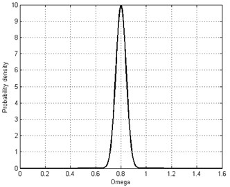
a) Rotation speed ()
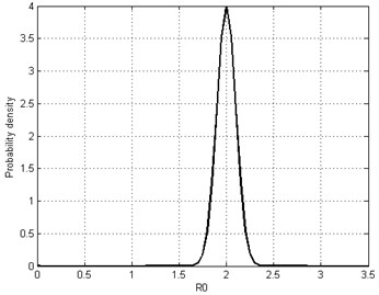
b) Clearance ()
It is easily found that the 99.7 % credible intervals are within the area of [0.6, 1]×[1.5, 2.5], so this area is approximate to substitute for the infinite bound for the normal distribution.
As discussed in section 3, the rotor/stator system will lose its stability through saddle-node bifurcation boundary (). Thus, the limit state function for this case is determined by the upper bound of saddle-node bifurcation as Eq. (25) and present in Fig. (4):
The reliability is defined as the probability that this system works stable (in safe region) as Eq. (26). By generating 1×10⁶ samples, it is calculated as 0.4195 through Monte-Carlo method. The safe/failure domain is intuitively depicted in Fig. 4:
In this scenario, only the stochastic information is considered, which is similar to previous research works considering uncertainties [20-22]. If other type uncertain information (e.g. interval) becomes available, the likelihood-based approach is adopted to perform an accurate reliability analysis.
5.2. Case 2. Pure epistemic uncertainty (single interval)
In this case, the effect to system response is investigated taking epistemic uncertainty into account. Both rotation speed and clearance are present in the interval form as [0.6, 1], [1.5, 2.5].
Fig. 4Safe region and failure region for case 1
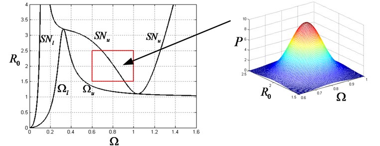
Fig. 5Safe region and failure region for case 2
Since it is equal the chance of uncertain variable and that take any arbitrary value within the given intervals, the reliability can be expressed as the ratio of the area for safe region and that for whole interval region. The reliability is thus analytical derived as Eq. (27) and the safe region/failure region is also present in Fig. 5:
where and correspond to the length of given interval for and .
5.3. Case 3. Mixed uncertainties (single interval)
For this scenario, the rotation speed is given as a random variable while the friction coefficient is present as an interval variable. Specific, and [0.1, 0.2].
Since no additional information is available for , the uniform distribution is adopted to model the friction coefficient as . The joint PDF is constructed as Eq. (28) and present in Fig. 6:
By setting other parameter fixed, the reliability is calculated as 0.4302 by drawing enough samples.
5.4. Case 4. Mixed uncertainties (multiple intervals)
In this case, the rotation speed remains unchanged as a random variable while the friction is given by multiple intervals: source 1: [0.05, 0.1], source 2: [0.1, 0.15], source 3: [0.15, 0.2], source 4: [0.2, 0.3].
By adopting the algorithm discussed in Section 4.4, the converted PDF is constructed as:
and shown in Fig. 7.
Fig. 6Safe region and failure region for case 3
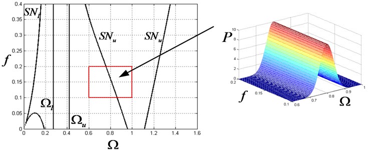
Fig. 7Safe region and failure region for case 4
The reliability is finally obtained as 0.4165 by generating enough samples.
5.5. Case 5 Mixed uncertainties (multiple intervals with spares data)
In this case, the uncertainties in , and are all taken into consideration. All available information listed in Table 3 is utilized to perform a credible reliability analysis.
The rotation speed is given in stochastic form, thus no further transformation needs to take. To the uncertainty in , the multiple input intervals from different sources can be dealt in similar way as case 4, so that samples can be easily generated from the PDF converted. In this case, we are focused on the uncertainty in .
Based on the accumulated knowledge, the uncertain parameter is assumed to follow one certain distribution (Normal) while the collected sparse data could be used to evaluate unknown statistic parameters ( and ). By adopting Bayesian rule, the likelihood of unknown parameters and is constructed as Eq. (29):
where and denote the PDF and CDF of normal distribution respectively. is the parameter vector, for this case , 3.
Since there is no additional available information, the non-informative prior is assigned as , , thus ) can be taken out of integration and the posterior joint PDF is reduced to:
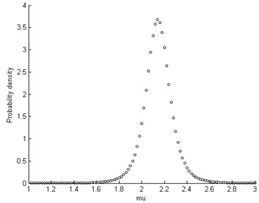
There is usually no analytical solution for Eq. (30), so the posterior joint PDF is numerical evaluated. The marginal distributions of the parameter and are depicted in Fig. 8.
Fig. 8PDF of mean and standard deviation
a) Mean of ()
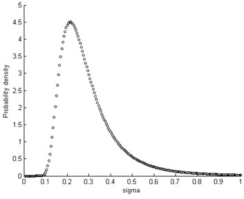
b) Standard deviation of ()
Fig. 9Unconditional PDF of R0
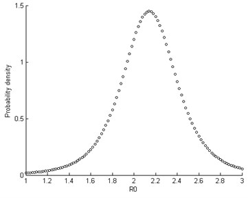
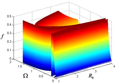
Fig. 10Limit state surface on the space of Ω, R0 and f
The unconditional PDF is obtained by integrating over the space of parameters as:
Fig. (9) presents the unconditioned posterior PDF of variable .
The reliability is finally calculated as 0.6142 and the limit state surface is shown in the parameter space (, and ) as Fig. 10.
It should be noted that even if the variable is assumed to follow a particular type of a parametric distribution (Normal), the unconditional density after the integration in Eq. (31) (where the uncertainty in the estimates of the parameters is accounted for) is non-parametric, i.e. the resultant probability distribution is not of the same type and cannot be classified as normal. See in Fig. 8.
6. Discussion
6.1. Benefits and achievements
In the context of uncertain dynamic analysis, the developed framework incorporates both deterministic data and uncertain information in a coherent way compared with different approaches for different kinds of data pursued in previous studies. This proposal is flexible and allows simultaneous processing of information in different formats, i.e. sparse point data, probability distribution and interval estimates, indicating a successful information aggregation and data fusion.
On the other hand, to achieve an accurate result, the system response function needs to be evaluated repeatedly to calculate the statistics of the output quantity. The uncertainties in both probability distribution and distribution parameters are included, which require a double loop sampling process. This procedure is cumbersome and may lead to extensive computation for large sample numbers. In the proposed approach, the computation cost is significantly reduced as the double loop sampling is collapsed into a single loop by discarding traditional Monte Carlo method. A unique PDF is constructed which is convenient for further dynamic analysis or risk assessment.
6.2. Validation and verification
It is found that the reliability analysis result differs significantly with different sources of uncertainty (case 1, 2 vs. case 3, 4) or representation of uncertainty in different formats (case 1 vs. case2, case 3 vs. case 4) taken into account, indicating a subtle influence of different uncertain variables to the outcome. Though these calculation results are derived based on numerical simulation, it still has profound significance in practical engineering. For example, the safe region obtained is smaller than expected when taking all possible uncertain factors into consideration. It is desired to increase the original clearance under deterministic situation for a safer rotor/stator design as rotating speed continues increasing. It should also be noticed that the calculation result (e.g. reliability) is only a reference value for an individual unit. Since the information used is given in statistical form (probability distribution), the result can only be experimentally validated under the circumstance with enough large samples.
7. Conclusions
In this paper, a modified Jeffcott rotor/stator system with mixed uncertainties is taken into study. The concept of likelihood is extended from classical point value to interval variables, which lay the foundation of proposed algorithm for PDF construction under mixed uncertainty. A likelihood-based approach addressing multiple inputs is developed, which enable a comprehensive uncertain dynamic analysis to the rotor/stator system incorporating all available information (sparse point data, probabilistic distribution and intervals). Several numerical cases are presented for demonstration and validation. Since the coexistence of both aleatory uncertainty and epistemic uncertainty is inevitable in practical engineering, the developed methodology has an extensive application prospect, such as industry manufacturing & mounting, risk assessment and product maintaining.
References
-
Black H. F. Interaction of a whirling rotor with a vibrating stator across a clearance annulus. International Journal of Mechanical Engineering Science, Vol. 10, 1968, p. 1-12.
-
Muszynska A. Synchronous self-excited rotor vibration caused by a full annular rub. Machinery Dynamics 8th Seminar, Halifax, Nova Scotia, Canada, Canadian Machinery Association, 1984, p. 1-21.
-
Muszynska A. Rotor-to-stationary element rub-related vibration phenomena in rotating machinery – literature survey. Sound and Vibration, Vol. 21, Issue 3, 1989, p. 3-11.
-
Bently D. E., Goldman P., Yu J. J. Full annular rub in mechanical seals. Part II: analytical study. Proceedings of ISROMAC-8, Honolulu, Hawaii, USA, 2000.
-
Jiang J., Ulbrich H. Stability analysis of sliding whirl in a nonlinear Jeffcott rotor with cross-coupling stiffness coefficients. Nonlinear Dynamics, Vol. 24, Issue 3, 2001, p. 269-283.
-
Childs D. W. Rub-induced parametric excitation in rotors. Journal of Mechanical Design, Vol. 101, 1979, p. 640-644.
-
Childs D. W. Fractional-frequency rotor motion due to non-symmetric clearance effects. Journal of Engineering for Power, Vol. 104, 1982, p. 533-541.
-
Ehrich F. F. High order subharmonic response of high speed rotors in bearing clearance. ASME Journal of Vibration, Acoustics, Stress, and Reliability in Design, Vol. 110, 1988, p. 9-16.
-
Day W. B. Asymptotic expansions in nonlinear rotor dynamics. Quarterly of Applied Mathematics, Vol. 44, Issue 4, 1987, p. 779-792.
-
Kim Y. B., Noah S. T. Quasi-periodic response and stability analysis for a nonlinear Jeffcott rotor. Journal of Sound and Vibration, Vol. 190, Issue 2, 1996, p. 239-253.
-
Choi S. K., Noah S. T. Mode-locking and chaos in a Jeffcott rotor with bearing clearances. ASME Journal of Applied Mechanics, Vol. 61, 1994, p. 131-138.
-
Goldman P., Muszynska A. Chaotic behavior of rotor/stator system with rubs. Journal of Engineering for Gas Turbins and Power, Vol. 116, 1994, p. 693-701.
-
Chu F., Zhang Z. Bifurcation and chaos in a rub-impact Jeffcott rotor system. Journal of Sound and Vibration, Vol. 210, Issue 1, 1998, p. 1-18.
-
Zhang W. Dynamic instability of multi-degree-of-freedom flexible rotor systems due to full annular rub. IMechE, 1988, p. 305-308.
-
Crandall S. From whirl to whip in rotor dynamics. Transactions of IFToMM 3rd International Conference on Rotor dynamics, Éd. du Centre NatiScient, 1990, p. 19-26.
-
Bartha A. R. Dry friction backward whirl of rotors: theory, experiments, results, and recommendations. 7th International Symposium on Magnetic Bearings, ETH Zurich, Schwitzland, 2000.
-
Bently D. E., Yu J. J., Goldman P. Full annular rub in mechanical seals. Part I: experimental results. Proceedings of ISROMAC-8, Honolulu, Hawaii, USA, 2000.
-
Jiang J., Ulbrich H. The physical reason and the analytical condition for the onset of dry whip in rotor-to-stator contact systems. Journal of Acoustics and Vibration – Transactions of the ASME, Vol. 127, 2005, p. 594-603.
-
Jiang J. The analytical solution and existence condition of dry friction backward whirl in rotor-to-stator contact systems. Journal of Acoustics and Vibrations – Transactions of the ASME, Vol. 129, 2007, p. 260-264.
-
Liao Haitao Global resonance optimization analysis of nonlinear mechanical systems: application to the uncertainty quantification problems in rotor dynamics. Communications in Nonlinear Science and Numerical Simulation, Vol. 19, Issue 9, 2014, p. 3323-3345.
-
Didier Jérome, Jacques Jean Sinou, Faverjon Béatrice Study of the non-linear dynamic response of a rotor system with faults and uncertainties. Journal of Sound and Vibration, Vol. 331, Issue 3, 2012, p. 671-703.
-
Jean-Jacques Sinou, Faverjon Béatrice The vibration signature of chordal cracks in a rotor system including uncertainties. Journal of Sound and Vibration, Vol. 331, Issue 1, 2012, p. 138-154.
-
Motley Michael R., Young Yin L. Influence of uncertainties on the response and reliability of self-adaptive composite rotors. Composite Structures, Vol. 94, Issue 1, 2011, p. 114-120.
-
Lingener A. Experimental investigation of reverse whirl of a flexible rotor. Transactions of IFToMM 3rd International Conference on Rotor dynamics, Lyon, France, 1990, p. 13-18.
-
Wu F., Flowers G. T. An experimental study of the influence of disk flexibility and rubbing on rotor dynamics. ASME, Vibration of Rotating Systems, Vol. 60, 1993, p. 19-26.
-
Helton J. C. Quantification of margins and uncertainties: conceptual and computational basis. Reliability Engineering and System Safety, Vol. 96, 2011, p. 976-1013.
-
Helton J. C. Quantification of margins and uncertainties: alternative representations of epistemic uncertainty. Reliability Engineering and System Safety, Vol. 96, 2011, p. 1034-1052.
-
Helton J. C., Johnson J. C., Sallaberry C. J. Quantification of margins and uncertainties: example analyses from reactor safety and radioactive waste disposal involving the separation of aleatory and epistemic uncertainty. Reliability Engineering and System Safety, Vol. 96, 2011, p. 1014-33.
-
Zaman Kais, Rangavajhala Sirisha, McDonald Mark P., Mahadevan Sankaran A probabilistic approach for representation of interval uncertainty. Reliability Engineering and System Safety, Vol. 96, 2011, p. 117-130.
-
Sankararaman Shankar, Mahadevan Sankaran Likelihood-based representation of epistemic uncertainty due to sparse point data and/or interval data. Reliability Engineering and System Safety, Vol. 96, 2011, p. 814-824.
-
Wallstrom Timothy C. Quantification of margins and uncertainties: a probabilistic framework. Reliability Engineering and System Safety, Vol. 96, 2011, p. 1053-1062.
-
Urbina Angel, Mahadevan Sankaran, Paez Thomas L. Quantification of margins and uncertainties of complex systems in the presence of aleatoric and epistemic uncertainty. Reliability Engineering and System Safety, Vol. 96, 2011, p. 1114-1125.
-
Edwards A. W. F. Likelihood. 1st Ed. Cambridge University Press, Cambridge, 1972.
-
Pawitan Y. In All Likelihood: Statistical Modeling and Inference Using Likelihood. Oxford Science Publications, New York, 2001.
-
Barnard G. A., Jenkins G. M., Winsten C. B. Likelihood inference and time series. Journal of the Royal Statistical Society, Series A, Vol. 125, 1962, p. 321-372.
Cited by
About this article

The authors gratefully acknowledge the financial support from the National Basic Research Program of China (973 Program, Project Number: 2013CB733000) and the National Natural Science Foundation of China (No. 51675026).
