Finite time point-stabilization of underwater spherical roving robot

Liu, Zhimin; Sun, Hanxu; Li, Yansheng; Jia, Qingxuan; Chu, Ming

doi:10.21595/jve.2016.16990

Journal of Vibroengineering

Browse Journal

Submit article

Published: 30 September 2016

Check for updates

Finite time point-stabilization of underwater spherical roving robot

Zhimin Liu¹

Hanxu Sun²

Yansheng Li³

Qingxuan Jia⁴

Ming Chu⁵

^{1, 2, 3, 4, 5}Institute of Automation, Beijing University of Posts and Telecommunications, Beijing 100876, China

Corresponding Author:

Zhimin Liu

Cite the article Download PDF

Downloads 1431

WoS Core Citations 2

CrossRef Citations 2

Abstract

This paper addresses the point stabilization problem for the underwater spherical roving robot (BYSQ-3) in the horizontal plane. The finite-time stable control laws are adopted to steer the robot to the origin fast, accurately and reliably. Firstly, the inner structure and operational principle of the robot is described and the kinematic and dynamic equations are established. Secondly, the diffeomorphism transformation and change of inputs are introduced to decouple the multivariable coupling system into two subsystems. The second subsystem consists of two double integrator systems. The finite-time controller is introduced to ensure part states converge to zero in finite time. Then, the other states are steered to the origin using the same method. Thirdly, the design process has no virtual input and the stability analysis is simple, the controller designed is easy for engineering implementation. The simulation and experiment results are presented to validate the shorter convergence time and better stability character of the controller.

1. Introduction

The past two decades has been witnessed the rapid development of various underwater autonomous unmanned vehicles(UAVs), with the help of the robotics, interacting with and exploring the underwater world becomes more feasible [1]. The underwater spherical robots, with the advantages such as good water pressure resistance, high concealment, flexible movement, zero turning radius, etc., have attracted many scholars and researchers’ attention. BYSQ-3 is the third-generation underwater spherical roving robot designed by Beijing University of Posts and Telecommunications (BUPT), in Fig. 1. BYSQ-3 is mainly used to perform the roles of deep-sea fixed-point photography and detection. To discharge the tasks，it is necessary to implement precise position and attitude for the UAV, that is, point stabilization problems. In fact, dynamic positioning and automatic docking in harbor can be classified as point stabilization problems. However, the UAVs generally are under-actuated mechanical system, which possess more degrees of freedom than the independent control inputs, it is impossible to implement accelerations in all DOF simultaneously [2]. Furthermore, the under-actuated UAVs’ kinematic and dynamic equations are highly coupled and strongly intrinsic nonlinear nature. On the horizontal plane, the UAV’s motion principle is similar to the surface vessels. Now, the planar point stabilization control study on the under-actuated UAVs and surface vessels has been a field of great interest to various researchers. See for example [3-7].

The under-actuated vehicles fail to meet the brocket’s theorem [8], no smooth or continuous time invariant control law can make the solution of the under-actuated UAVs’ kinematic and dynamic equations asymptotically stable. In order to realize the control objective, many scholars and researchers proposed non-smooth or continuous time-varying control laws. In [9], a time-varying switching control law was proposed to make the under-actuated surface vehicles $k$ -exponential stable. In [10], a discontinuous approach (TSM) was addressed to stabilize the under-actuated surface vessels. In [11], through the coordinates change, the dynamical system could be reduced to a third-order chained form, by using the time-invariant discontinuous state feedback law, the global asymptotic stabilization of the system could be guaranteed. In [12], a set-point controller was described for UAVs by using the transformed equations of motion. In [13], a logic-based hybrid controller was addressed which can guarantee the global asymptotic convergence to an arbitrarily small neighborhood of the origin. The control techniques used in the aforementioned literature have at best exponential convergence rate with infinite settling time, in other words, the under-actuated underwater vehicles converge to a final target point with a desired orientation in finite time is impossible. However, some tasks, for example, underwater search and rescue, detection and surveillance, etc., they are time sensitive, it is desirable the underwater robot can accomplish these tasks quickly in finite time rather than infinite asymptotically. The finite-time control laws possess many nice features such as faster convergence rates, higher accuracies and better disturbance rejection properties. Hence, the finite-time design methods for nonholonomic systems have attracted increasing attention worldwide. Particularly, by using the finite-time control method, the authors in [14] proposed the switched method to solve the point stabilization problems of the under-actuated underwater vessels, through a sequential series of switched control laws, each stage could achieve a certain objective, in the final the system could be steered to the origin. In [15], the trajectory tracking problem for under-actuated UAV in the horizontal plane was addressed, by adopting the finite-time tracking control laws, all the tracking errors of the UAV converged to the origin except for the yaw angular $r$ was BIBO stabilization. In [16], the output feedback stabilization for a class of under-actuated systems were investigated and the designed controller guarantees that the state variables converge to zero within finite time. In [17], the high-order uncertain nonlinear systems’ finite-time stabilization problem was investigated, by combining with adaptive technique, the convergent time can be adjusted arbitrarily by pre-assigning the design parameter. Many other researchers investigated the nonlinear under-actuated systems finite-time control problems, see for [18-21].

In this paper, the finite-time controller is introduced to ensure part states converge to zero in finite time, then the whole system can converge to zero fastly. Compared with the other traditional approaches, the proposed approaches have shorter convergence time and it is the minimum energy control strategy.

The paper is organized as follows. In Section 2, the inner structure and operational principle of the underwater spherical roving robot is described and the kinematic and dynamic equations are established based on Newton Euler equations. In Section 3, the finite time control laws are designed and the finite-time stability property is analyzed. In Section 4, 5, the simulation and experiment results are depicted and analyzed. Section 6 provides the conclusions.

2. Description of the control problem

2.1. The structure of BYSQ-3

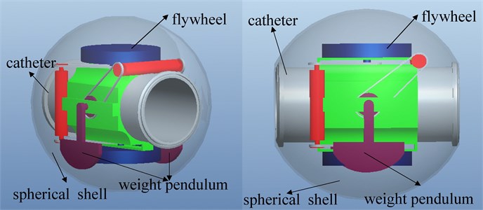
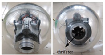
BYSQ-3 is a novel underwater spherical roving robot with only one propeller located in the middle of the catheter, its posture can be adjusted through heavy pendulum and the flywheel. The catheter is fixedly connected with the spherical shell. The sleeve (generally called long axis or the rolling axis) is mounted the outer wall of the conduit and it can rotate around the catheter. The short axis (or pitching axis) is fixedly connected with the sleeve and perpendicular to the long axis. The weight pendulum mechanism is installed on both ends of the short axis. Driven by the long axis motor, the weight pendulum can rotate around the catheter and the robot’s roll angle can change. Driven by the short axis motor, the weight pendulum can swing around the short axis and the robot’s pitch angle can change. Driven by the flywheel motor, the robot body get the anti-force to change the yaw angle. The serve motors and control circuits were sealed inside the spherical glass fiber hull to reduce the possible damage. The three-dimensional structure chart of BYSQ-3 are shown in Fig. 1. In the horizontal plane, the control inputs are propeller thrust and steering torque provided by the flywheel.

Fig. 1Three-dimensional structure chart

2.2. Kinematics and dynamics of BYSQ-3

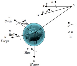
The inertial and the body-fixed reference frame is shown in Fig. 2. The kinematic and dynamic equations of BYSQ-3 in horizontal plane can be written as Eq. (1) [2]:

1

\{\begin{array}{l} \begin{array}{l} \dot{x} = u c o s φ - v s i n φ, \\ \dot{y} = u s i n φ + v c o s φ, \\ \dot{φ} = r, \end{array} \\ \begin{array}{l} \dot{u} = \frac{(m_{22} v r - d_{11} u + τ_{1})}{m_{22}}, \\ \dot{v} = - \frac{(m_{11} u r + d_{22} v)}{m_{22}}, \\ \dot{r} = \frac{((m_{11} - m_{22}) u v - d_{33} r + τ_{3})}{m_{33}}, \end{array} \end{array}

where $x$ , $y$ and $φ$ denote the position and orientation (yaw angle) of BYSQ-3 in the inertial frame, $u$ , $v$ and $r$ represent the linear surge, sway and angular velocities of BYSQ-3 in the body- fixed frame. $m_{i i}$ , $d_{i i}$ , $i =$ 1, 2, 3 represent the inertia including added mass effects and hydrodynamic coefficients of the drag terms. $τ_{1}$ , $τ_{3}$ represent the external force and torque generated by propeller and flywheel, there is no sway thruster, thus, the 3 DOFs’ horizontal motion must be controlled by the two independent control input, so, Eq. (1) is an under-actuated control system.

Assumption: (i) The spherical shell is a perfect spherical with homogeneous mass distribution. (ii) The heave, pitch, and roll motions are neglected and the effects of wave, wind and current are ignored.

Fig. 2The inertial and the body-fixed reference frame

2.3. Control objective

The control objective is to deal with the problem to move the underwater spherical roving robot BYSQ-3 from one motion point to another point. Without loss of generality，the control problem can be described as the stabilization of the nonlinear dynamical system to the origin from a nonzero initial condition.

3. Design of the control system

3.1. Mathematical preliminaries

Definition 1 [22]. Consider a nonlinear dynamical system:

2

\dot{x} (t) = f (x (t)) = {[f_{1} (x), f_{2} (x), \dots, f_{n} (x)]}^{T},

where $f : R^{n} \to R^{n}$ is continuous vector field and $f (0) = 0$ , $R^{n}$ denotes the $n \times 1$ column vectors set. The zero solution $x (t) = 0$ of system Eq. (2) is finite time stable means that an open neighborhood $U \in R^{n}$ of the origin exists and the following statements hold

(i) Lyapunov stability.

(ii) Finite-time convergence. That is, for every $t_{0} \in [0, \infty)$ and $x (t_{0}) = x_{0} \in U$ , there exists a settling-time function $T (t_{0}, x_{0})$ , for all $t \in [t_{0}, T]$ , every solution $x (t; t_{0}; x_{0})$ of the dynamical system (2) satisfies $\lim_{t \to T} x (t; t_{0}; x_{0}) = 0$ and for all $t \in [T, \infty]$ , $x (t; t_{0}; x_{0}) = 0$ . If $U = R^{n}$ , the zero solution $x (t) = 0$ of Eq. (2) is globally finite-time stable.

Definition 2 [23]. Consider the continuous vector field $f (x (t))$ of Eq. (2), it is called homogeneous of degree $k$ with respect to $r_{1}$ ,…, $r_{n}$ , if there exists positive real numbers $r_{1}$ ,…, $r_{n}$ , such that $f_{i} (ε^{r_{1}} x_{1}, \dots, ε^{r_{n}} x_{n}) = f_{i} (x) ε^{k + r_{i}}$ for all $ε > 0$ , where $k \geq - \max (r_{i})$ , $i =$ 1,…, $n .$

Lemma 1 [23]. System (1) is global finite-time stable if it is globally asymptotically stable and is homogeneous with a negative degree $k$ . Throughout this paper, the foregoing definitions and Lemma 1 help to derive the main result.

3.2. Design of the finite time control law

To simplify the controller design, firstly the system Eq. (1) is decoupled by the coordinate transformation, define:

{[z_{1}, z_{2}, z_{3}, z_{4}, z_{5}, z_{6}]}^{T} = T {[x, y, φ, u, v, r]}^{T},

where $T$ is a partitioned matrix, and:

T_{11} = (\begin{matrix} c o s φ & s i n φ & 0 \\ - s i n φ & c o s φ & 0 \\ 0 & 0 & 1 \end{matrix}), T_{21} = (\begin{matrix} - c o s φ & - s i n φ & 0 \\ 0 & 0 & 0 \\ 0 & 0 & 1 \end{matrix}),

T_{12} = d i a g (0, \frac{m_{22}}{d_{22}}, 0), T_{22} = d i a g (- \frac{m_{11}}{d_{22}}, 1,1) .

From the structure of $T$ , it is easy to see $|T| = |T_{11}| |T_{22}| \neq 0$ , hence, $T$ is a reversible transformation, stabilization of the vector ${[x, y, φ, u, v, r]}^{T}$ can be changed into stabilizing the vector ${[z_{1}, z_{2}, z_{3}, z_{4}, z_{5}, z_{6}]}^{T}$ . Based on the coordinate transformation, define:

\frac{((d_{11} - d_{22}) u - d_{22} z_{2} z_{6} - τ_{1})}{d_{22}} = F_{1}, \frac{((m_{11} - m_{22}) u v - d_{33} r + τ_{3})}{m_{33}} = F_{2}

a = \frac{d_{22}}{m_{11}}, b = \frac{m_{22}}{d_{22}}, c = \frac{d_{22}}{m_{22}} .

$F_{1}$ , $F_{2}$ are considered as new inputs to be designed later.

Using the above change of coordinates, the kinematic and dynamic Eq. (1) of BYSQ-3 can be written as the following two subsystems:

3

\{\begin{array}{l} {\dot{z}}_{1} = - a z_{1} - a z_{4} + z_{2} z_{6} - b z_{5} z_{6}, \\ {\dot{z}}_{5} = - c z_{5} - c z_{6} (z_{1} + z_{4}), \end{array}

4

\{\begin{array}{l} \begin{array}{l} {\dot{z}}_{2} = z_{4} z_{6}, \\ {\dot{z}}_{3} = z_{6}, \end{array} \\ \begin{matrix} {\dot{z}}_{4} = F_{1}, \\ {\dot{z}}_{6} = F_{2} . \end{matrix} \end{array}

We assume the initial value of $z_{6}$ satisfies $z_{6} (0) \neq 0$ , the design of the control laws can be divided into three stages.

Stage 1. The objective of this stage is to steer $z_{2}$ , $z_{4}$ to zero in finite time $T_{1}$ and we set $F_{2} = 0$ for this stage.

Theorem 1. Consider the following nonlinear subsystem of Eq. (4):

5

\{\begin{array}{l} {\dot{z}}_{2} = z_{4} z_{6}, \\ {\dot{z}}_{4} = F_{1} . \end{array}

The following state feedback control law:

6

\{\begin{array}{l} F_{1} = \frac{- k_{1} s i g n {|z_{2}|}^{α_{1}} - k_{2} s i g n (z_{4} z_{6}) {|z_{4} z_{6}|}^{α^{2}}}{z_{6}}, \\ F_{2} = 0, \end{array}

where $k_{1} > 0$ , $k_{2} > 0$ , $0 < α_{1} < 0$ , $α_{2} = 2 α_{1} / 1 + α_{1}$ can stabilize the system Eq. (6) in finite time $T_{1}$ .

Proof: Based on Lemma 1, the proof of this theorem is divided into two steps:

Step 1 (Asymptotically stable). Consider the candidate Lyapunov function:

V (z_{2}, z_{4}) = k_{1} \frac{{|z_{2}|}^{1 + α_{1}}}{(1 + α_{1})} + \frac{1}{2} {(z_{4} z_{6})}^{2},

its time-derivative along the system Eq. (6) renders to:

\dot{V} (z_{2}, z_{4}) = k_{1} s i g n {|z_{2}|}^{α_{1}} z_{4} z_{6} + z_{4} z_{6} (k_{1} s i g n (z_{2}) {|z_{2}|}^{α_{1}}

- k_{2} s i g n (z_{4} z_{6}) {|z_{4} z_{6}|}^{α_{2}} = - k_{2} {|z_{4} z_{6}|}^{α_{2}} \leq 0 .

So the $\dot{V} (z_{2}, z_{4})$ is negative, and the $V (z_{2}, z_{4})$ is monotony decrease. From the definition of $V (z_{2}, z_{4})$ , we have $0 < V (z_{2}, z_{4}) < V (z_{2} (0), z_{4} (0)) < \infty$ , thus $V (z_{2}, z_{4})$ is bounded, and so its arguments $z_{2}$ , $z_{4}$ must be bounded.

The second-order time-derivative of $V (z_{2}, z_{4})$ along the system Eq. (6) renders to:

\ddot{V} (z_{2}, z_{4}) = - k_{2} (1 + α_{2}) s i g n (z_{4} z_{6}) {|z_{4} z_{6}|}^{α_{2}} .

Since $z_{4}$ is bounded, we get that $\ddot{V} (z_{2}, z_{4})$ is bounded, then $\dot{V} (z_{2}, z_{4})$ is uniformly continuous. from the Barbalat Lemma [24], we can get:

\lim_{t \to \infty} \dot{V} (z_{2}, z_{4}) = - k_{2} {|z_{4} z_{6}|}^{α_{2}} = 0 .

Remembering that $F_{2} = 0,$ from the Eq. (4), we have $z_{6} (t) \equiv z_{6} (0) \neq 0,$ then $\lim_{t \to \infty} \dot{V} (z_{2}, z_{4}) = 0$ is equivalent to:

7

\lim_{t \to \infty} z_{4} = 0 .

To proof that $\lim_{t \to \infty} z_{2} = 0$ , substituting $F_{1}$ into Eq. (5), considering the function $z_{2} z_{4}$ and its time-derivative along the system Eq. (5):

\frac{d (z_{2} z_{4})}{d t} = - k_{1} \frac{{|z_{2}|}^{{1 + α}_{1}}}{z_{6}} - \frac{k_{2} s i g n (z_{4} z_{6}) {|z_{4} z_{6}|}^{α_{2}} + z_{4}^{2} z_{6}}{z_{6}} .

Let:

p_{1} (t) = - k_{1} \frac{{|z_{2}|}^{{1 + α}_{1}}}{z_{6}}, p_{2} (t) = \frac{k_{2} s i g n (z_{4} z_{6}) {|z_{4} z_{6}|}^{α_{2}} + z_{4}^{2} z_{6}}{z_{6}} .

Remembering that $z_{6} (t) \equiv z_{6} (0) \neq 0,$ $z_{2}$ is bounded, we can get ${\dot{p}}_{1} (t)$ is bounded and uniformly continuous. From $\lim_{t \to \infty} z_{4} = 0$ , we have $\lim_{t \to \infty} p_{2} (t) = 0$ , from the Barbalat Lemma, we can get $\lim_{t \to \infty} p_{1} (t) = 0$ , it is equivalent to:

8

\lim_{t \to \infty} z_{2} = 0 .

From Eqs. (7) and (8), there exist state feedback law Eq. (6) which globally asymptotically stabilize $z_{2}$ , $z_{4}$ to the origin.

Step 2 (Negative homogeneous degree). Let:

f (z_{2}, z_{4}) = {[f_{1} (z_{2}, z_{4}), f_{2} (z_{2}, z_{4})]}^{T} = (\begin{matrix} z_{4} z_{6} \\ \frac{- k_{1} s i g n {|z_{2}|}^{α_{1}} - k_{2} s i g n (z_{4} z_{6}) {|z_{4} z_{6}|}^{α_{2}}}{z_{6}} \end{matrix}),

and choose $r_{1} = 1$ , $r_{2} = (1 + α_{1}) / 2$ , then:

f ({ε^{r_{1}} z}_{2}, {ε^{r_{2}} z}_{4}) = (\begin{matrix} f_{1} ({ε^{r_{1}} z}_{2}, {ε^{r_{2}} z}_{4}) \\ f_{2} ({ε^{r_{1}} z}_{2}, {ε^{r_{2}} z}_{4}) \end{matrix})

= (\begin{matrix} {ε^{r_{2}} z}_{4} z_{6} \\ \frac{- k_{1} s i g n {|{ε^{r_{1}} z}_{2}|}^{α_{1}} - k_{2} s i g n ({ε^{r_{2}} z}_{4} z_{6}) {|{ε^{r_{2}} z}_{4} z_{6}|}^{α_{2}}}{z_{6}} \end{matrix})

= (\begin{matrix} ε^{r_{1} + k} & 0 \\ 0 & ε^{r_{2} + k} \end{matrix}) (\begin{matrix} z_{4} z_{6} \\ \frac{- k_{1} s i g n {|z_{2}|}^{α_{1}} - k_{2} s i g n (z_{4} z_{6}) {|z_{4} z_{6}|}^{α_{2}}}{z_{6}} \end{matrix}),

where $k = (α_{1} - 1) / 2 < 0 .$

Based on step 1, we know that system Eq. (5) is global asymptotically stable, from step 2, we know that the system Eq. (5) is homogeneous with a negative degree $k$ based on Lemma 1, system Eq. (5) is global finite-time stable.

Since the system Eq. (5) is global finite-time stable under the control law Eq. (6), hence there exists time $T_{1}$ , $\forall t \geq T_{1}$ , $z_{2} (t) = z_{4} (t) = 0$ and $F_{1} = 0$ . If we render $F_{2} \neq 0$ at time $T_{1}$ , then the change of $F_{2}$ affect the state variable $z_{3}$ , $z_{6}$ while $z_{2}$ , $z_{4}$ remains unaffected due to the dynamics of the system Eq. (4).

Stage 2. The objective of this stage is to steer $z_{3}$ , $z_{6}$ to zero in finite time $T_{2}$ , we set $F_{1} = 0$ for this stage, in particular, this stage we proof $z_{1}$ , $z_{5}$ is bounded when $t \leq T_{1} + T_{2}$ , there is no finite time escape phenomenon for $z_{1}$ , $z_{5}$ .

Now consider the subsystem:

9

\{\begin{array}{l} {\dot{z}}_{3} = z_{6}, \\ {\dot{z}}_{6} = F_{2}, \end{array}

it is a double integrator system similar to system Eq. (6), to regulate $z_{3}$ , $z_{6}$ to zero in finite time $T_{2}$ , the following control law Eq. (10) is applied to system Eq. (9):

10

\{\begin{array}{l} F_{1} = 0, \\ F_{2} = - k_{3} s i g n {|z_{3}|}^{α_{3}} - k_{4} s i g n (z_{6}) {|z_{6}|}^{α_{4}}, t \geq T_{1} . \end{array}

Theorem 2. The following switching control law:

\{\begin{array}{l} F_{1} = \frac{- k_{1} s i g n {|z_{2}|}^{α_{1}} - k_{2} s i g n (z_{4} z_{6}) {|z_{4} z_{6}|}^{α^{2}}}{z_{6}}, \\ F_{2} = 0, t \leq T_{1} \end{array}

\{\begin{array}{l} F_{1} = 0, \\ F_{2} = - k_{3} s i g n {|z_{3}|}^{α_{3}} - k_{4} s i g n (z_{6}) {|z_{6}|}^{α_{4}}, t \geq T_{1} . \end{array}

Moves the states $z_{2}$ , $z_{3}$ , $z_{4}$ , $z_{6}$ to zero in finite-time $T_{1} + T_{2}$ and at the end of which we have $z_{2} (t) = {z_{3} (t) = z_{4} (t) = z}_{6} (t) = 0$ , the state variable $z_{1}$ , $z_{5}$ is bounded and the closed-loop system is globally finite-time stable.

Proof: From the above control law, the state variable $z_{2}$ , $z_{4}$ converge to zero at time $T_{1}$ , when $t \geq T_{1}$ , the change of $F_{2}$ affect the state variable $z_{3}$ , $z_{6}$ while $z_{2}$ , $z_{4}$ remains unaffected, below we illustrate there don’t exist finite – time escape phenomenon for $z_{3}$ , $z_{6}$ , when $t \in [0, T_{1}]$ , $F_{2} = 0$ , from ${\dot{z}}_{6} = F_{2}$ , $z_{6}$ will be a constant value ( $z_{6} (t) = z_{6} (0)$ ), from ${\dot{z}}_{3} = z_{6}$ , we know $z_{3}$ exhibits a linear increase with time and is bounded. From the design of the control law, we have $z_{2} (t) = {z_{3} (t) = z_{4} (t) = z}_{6} (t) = 0,$ for all $t > T_{1} + T_{2}$ in fact, $z_{1},$ $z_{5}$ is bounded for all $t \in [0, T_{1} + T_{2}]$ .

Define the Lyapunov function:

V = \frac{d_{22}}{{2 m}_{22}} z_{1}^{2} + \frac{m_{22}}{d_{22}} z_{5}^{2},

then:

\dot{V} = \frac{d_{22}}{{2 m}_{22}} z_{1} {\dot{z}}_{1} + \frac{m_{22}}{d_{22}} z_{5} {\dot{z}}_{5} = \frac{d_{22}}{{2 m}_{22}} z_{1} (- \frac{d_{22}}{m_{11}} z_{1} - \frac{d_{22}}{m_{11}} z_{4} + z_{2} z_{6} - \frac{m_{22}}{d_{22}} z_{5} z_{6})

+ \frac{m_{22}}{d_{22}} z_{5} (- \frac{d_{22}}{m_{22}} z_{5} - \frac{d_{22}}{m_{22}} z_{6} (z_{1} + z_{4}))

= - \frac{d_{22}^{2}}{m_{11} m_{22}} z_{1}^{2} - z_{5}^{2} - z_{1} (\frac{d_{22}^{2}}{m_{11} m_{22}} z_{4} - \frac{d_{22}}{m_{22}} z_{2} z_{6}) + z_{4} z_{5} z_{6} .

From:

V = \frac{d_{22}}{{2 m}_{22}} z_{1}^{2} + \frac{m_{22}}{d_{22}} z_{5}^{2},

we have:

|z_{1}| \leq \sqrt{\frac{{2 m}_{22}}{d_{22}}} \sqrt{V}, |z_{5}| \leq \sqrt{\frac{{2 d}_{22}}{m_{22}}} \sqrt{V} .

Recalling that $z_{2} (t)$ , $z_{3} (t)$ , $z_{4} (t)$ , $z_{6} (t)$ is bounded for all $t \in [0, T_{2}]$ , we have:

\dot{V} \leq k_{1} V + k_{2} (t) \sqrt{V},

where:

k_{1} = \max (- \frac{d_{22}^{2}}{m_{11} m_{22}}, - 1), k_{2} (t) = (\frac{d_{22}^{2}}{m_{11} m_{22}} z_{4} - \frac{d_{22}}{m_{22}} z_{2} z_{6}) \sqrt{\frac{{2 m}_{22}}{d_{22}}} + z_{4} z_{6} \sqrt{\frac{{2 d}_{22}}{m_{22}}} .

Let $δ = \sqrt{V}$ , then:

\dot{δ} = \frac{d \sqrt{V}}{d t} \leq \frac{k_{1}}{2} δ + \frac{1}{2} k_{2} (t),

so:

δ (t) \leq e^{- \frac{1}{2} k_{1} T_{2}} δ (0) + \frac{1}{2} \int_{0}^{T_{2}} e^{- \frac{1}{2} k_{1} {(T}_{2} - t)} k_{2} (t) d t .

Recalling that $k_{2} (t)$ is bounded, so $z_{1}$ , $z_{5}$ is bounded for all $t \in [0, T_{2}]$ .

Stage 3. From the above analysis, when $t > T_{1} + T_{2}$ , the system becomes:

\{\begin{array}{l} {\dot{z}}_{1} = - a z_{1}, \\ {\dot{z}}_{5} = - c z_{5} . \end{array}

It is a Hurwitz system and is global uniform asymptotic stability.

4. System simulation

4.1. Control performance of the proposed method

In this section, a series of numerical simulation results are presented by using the MATLAB2014 /SIMULINK programs to illustrate the performance and of the tracking control laws. The results demonstrate that the tracking control laws can not only effectively achieve the trajectory tracking mission, the tracking control design is independent of the predefined desired trajectory. Specially, these control gains are $k_{1} =$ 4, $k_{2} =$ 10, $k_{3} =$ –0.2, $k_{4} =$ –0.3, $α_{1} =$ 0.5, $α_{2} =$ 2/3, $α_{3} =$ 0.3, $α_{4} =$ 6/13.

And the parameters: $m_{11} =$ 25 kg, $m_{22} =$ 25 kg, $m_{11} =$ 25 kg, $d_{11} =$ 0.4 kg/s, $d_{11} =$ 0.2 kg/s, $d_{11} =$ 0.001 kg/s.

The initial conditions are: $x (0) =$ 10 m, $y (0) =$ 10 m, $φ (0) = p i / 2$ , $u (0) =$ 1 m/s, $v (0) =$ 0 m/s, $r (0) =$ –0.1 rad/s.

The time-response of the states and the control inputs are shown in Fig. 3. The path traced by BYSQ-3 is shown in Figs. 4.

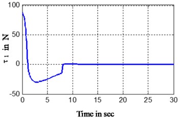
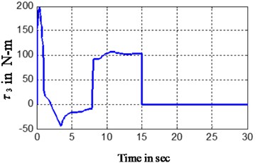
Fig. 3Simulation results of the finite time control laws

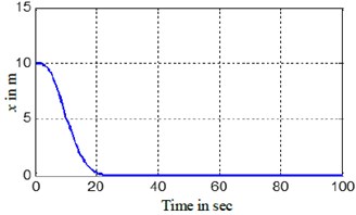
a) BYSQ-3x tracking

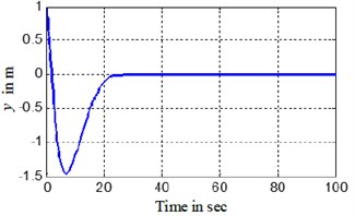
b) BYSQ-3y tracking

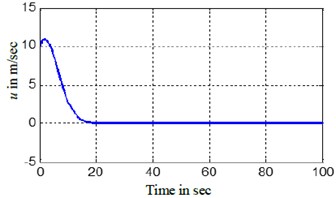
c) BYSQ-3u tracking

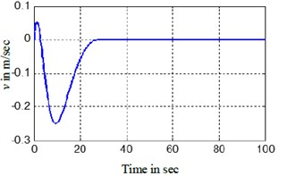
d) BYSQ-3v tracking

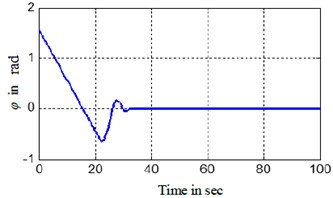
e) BYSQ-3 yaw angle

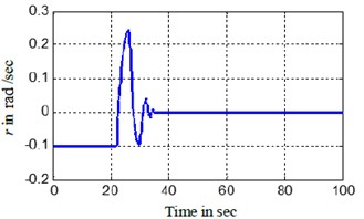
f) BYSQ-3 yaw angle velocity

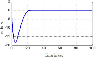
g) BYSQ-3 propeller thruster

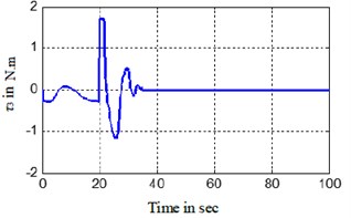
h) BYSQ-3 steering torgue

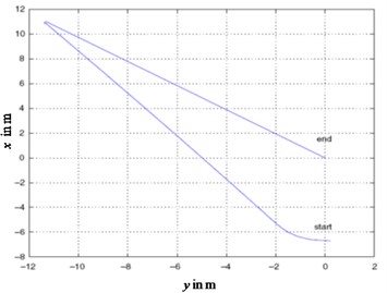
Fig. 4Actual trajectory of BYSQ-3

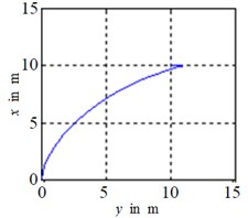
The Figs. 3, 4 show the position and orientation responses of the BYSQ-3, these results indicate that the position and orientation can fast converge to the origin in finite time. The position errors $x$ and $y$ are less than 0.08 m and e-5 during steady state, the orientation error is less than 10-3 degree. From the figures, it is easy to see the change slope of the sway velocity is less than that of the sway velocity, this is because there is no dependent control input in the sway, the sway motion is realized by using the couple effect of the surge and yaw. From Fig. 3(e), we know the angle change uniformly in the initial time. This is because the value of $F_{2}$ is zero and the angle velocity is a constant, the value of $F_{2}$ do not keep zero when $t > T_{1}$ until $t = T_{1} + T_{2}$ and the angle begin change, the flywheel can guarantee the effective of the effect. $g$ , $h$ of Fig. 3 illustrates the surge control force $τ_{1}$ and the yaw control torque $τ_{3}$ . Fig. 4 demonstrated the simulation trajectory of BYSQ-3 on the horizontal plane. From Fig. 4, the simulation trajectory of BYSQ-3 is similar to the motion of a car reverses to warehousing. In the initial time，BYSQ-3 has a forward deceleration behavior, then start reversing, reducing the yaw angle, and return to the origin the change process is relatively stable, and the overshoot is small. Above simulation results show that the designed finite time stabilization control law can effectively implement the underwater probe point stabilization control, convergence time is short, which will help to save energy.

4.2. Comparison with the finite time controller in [14]

In this subsection, the finite time control law proposed in this paper is compared with the finite time control law derived in [14], the initial conditions are: $x (0) =$ –3.7142 m, $y (0) =$ –3.8993 m, $φ (0) =$ 2 rad, $u (0) =$ 1 m/s, $v (0) =$ 3 m/s, $r (0) =$ –4 rad/s.

The gains of the control law proposed in this paper are: $k_{1} =$ 2.3, $k_{2} =$ 8, $k_{3} =$ –0.5, $k_{4} =$ –0.4, $α_{1} =$ 0.5, $α_{2} =$ 2/3, $α_{3} =$ 0.3, $α_{4} =$ 6/13.

The results are given in Figs. 5, 6, which compares the control torque，simulation trajectory by the controller in this paper and the controller in [14], it can be seen that the settling time consumed by the controller in [14] is over three times of that by controller in this paper, the control torque yields by the controller in [14] is relatively larger than that by controller in this paper because the controller in [14] yields a sudden sharp turn while the controller in this paper obtain a smooth motion curve, the distance travelled by the controller in [14] is relatively longer than that by controller in this paper. The numerical results show that the controller in this paper can save time and energy.

Fig. 5Simulation trajectory comparison of the two controllers

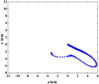
a) Controller in this paper

b) Controller in [14]

5. Experiment

The BYSQ-3 is a spherical underwater autonomous roving robot prototype that is 0.40 m diameter, and weighs about 30.6 kg in air (see Figs. 7, 8). The BYSQ-3 has an improved turning system structure resulting in better performance compared with BYSQ-2 [25]. In order to verify the performance of the control law proposed in this paper, we have conducted the experiments on the swimming pool in BUPT, china. at the end of December 2015, in the swimming pool there is no significant wind disturbance. The sensors are shown in Fig. 7.

Fig. 6Control torque comparison of the two controllers

a) Propeller thruster in this paper

b) Steering torque in this paper

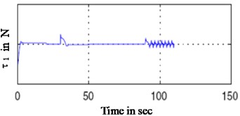
c) Propeller thruster [14]

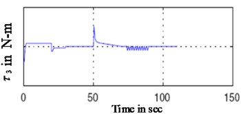
d) Steering torgue in [14]

Fig. 7The sensors of BYSQ-3: a) GY-80 nine-axis digital gyroscope, b) micronav navigation system, c) ultrasonic displacement sens, d) underwater camera

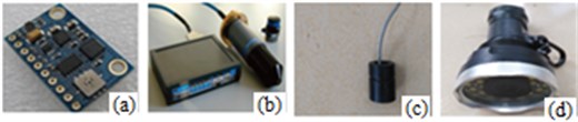
Fig. 8The prototype of BYSQ-3

BYSQ-3 uses real-time wireless remote control mode, the control structure is shown in Fig. 9, the controller adopts GD32F105 embedded computer, control software adopts the VxWorks real-time operating system, the time period for receiving and processing navigation and position data is 200 ms, and the movement state information is sent to the host computer through the communication module, the Control software was developed under visual studio 2012. The host computer starts a control cycle when receiving the robot’s state information and sent the drive instructions to the robot controller, the instructions were converted into output voltage signal to realize the motion control.

In the experimental process, the actual input signals is the input voltage while not the propeller thruster and the flywheel driving torque in the simulation process, to determine the relationship between motor input voltage and propeller thruster we measured the output thrust and torque under different voltages for 20 times. Through analyzing the experiment results, we found force-voltage relationships a quadratic parabolic at voltages with slightly different in the forward and backward stages. According to the experiment results, the input voltage of propeller thruster and the flywheel driving torque was shown in Figs. 10, 11.

Fig. 9Control structure of BYSQ-3

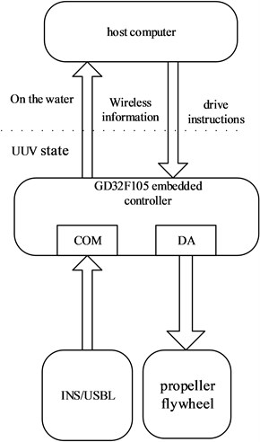
Fig. 10Change of input voltage of propeller

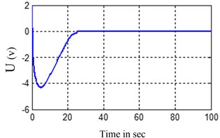
Fig. 11Change of input voltage of flywheel motor

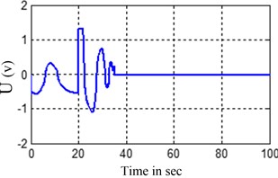
Fig. 12Underwater motion picture of BYSQ-3

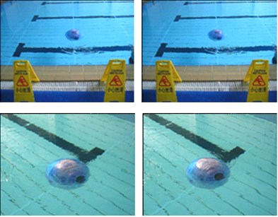
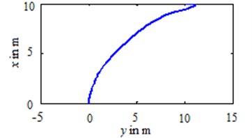
Fig. 13 is the actual trajectory based on the experiment data, and from experiment data, we can find the distance between the terminal point of BYSQ-3 and the origin is 0.27 m, the result is better than expected.

Fig. 13Actual trajectory of BYSQ-3

6. Conclusions

In this paper, we deal with the point stabilization problem of a novel underwater spherical roving robot BYSQ-3. the finite time stabilization controller is designed which can reduce the coupling degree and improve convergence rate of the system. As can be seen from the design process, there is no virtual input, which can improve the processing speed of the computer, Simulation results demonstrate the good performance of the control laws, the designed control laws can save time and therefore can save energy, the experimental results and simulation results have consistency.

References

Ehsan Peymani, Thor I. Fossen Path following of underwater robots using Lagrange multipliers. Robotics and Autonomous Systems, Vol. 67, 2015, p. 44-52.

Publisher
Do K. D., Pan J. Control of Ships and Underwater Vehicles. Advances in Industrial Control, 2009.

Publisher
Sans-Muntadas A., Brekke E. F., Øyvind Hegrenaes, et al. Navigation and probability assessment for successful AUV docking using USBL. Ifac Papersonline, Vol. 48, Issue 16, 2015, p. 204-209.

Publisher
Hegrenas O., Gade K., Hagen O. K., et al. Underwater transponder positioning and navigation of autonomous underwater vehicles. Oceans IEEE, 2009, p. 1-7.

Publisher
Palomeras N., Ridao P., Ribas D., et al. Autonomous I-AUV docking for fixed-base manipulation. 19th World Congress of the International Federation of Automatic Control, 2014, p. 12160-12165.

Publisher
Shigekuni T., Takimoto T. Stabilization of uncertain equilibrium points by dynamic state-derivative feedback control. 13th International Conference on Control, Automation and Systems, 2013, p. 23-27.

Publisher
Greytak M., et al. Underactuated point stabilization using predictive models with application to marine vehicles hover intelligent robots and systems. IEEE/RSJ International Conference, 2008, p. 3756-3761.

Publisher
Brockett R. W. Asymptotic stability and feedback stabilization. Differential Geometry for Nonlinear Control Theory, Vol. 27, 1983, p. 181-191.

Search CrossRef
Borhaug E, Pettersen K. Y. Adaptive way-point tracking control for underactuated autonomous vehicles. 44th Decision and Control, 2005 and 2005 European Control Conference, 2006, p. 4028-4034.

Search CrossRef
Cheng J., Yi J., Zhao D. Stabilization of an underactuated surface vessel via discontinuous control. Proceedings of the American Control Conference, 2007, p. 206-211.

Publisher
Ghommam J., Mnif F., Benali A., et al. Asymptotic backstepping stabilization of an underactuated surface vessel. Control Systems Technology IEEE Transactions, Vol. 14, Issue 6, 2006, p. 1150-1157.

Publisher
Przemysaw Herman Decoupled PD set-point controller for underwater vehicles. Ocean Engineering, Vol. 36, 2009, p. 529-534.

Publisher
Aguiar A. P., Pascoal A. M. Global stabilization of an underactuated autonomous underwater vehicle via logic-based switching. Proceedings of the 41st IEEE Conference on Decision and Control, Las Vegas, NE, USA, 2002, p. 3267-3272.

Publisher
Sankaranarayanan V., Mahindrakar A. D., Banavar R. N. A switched controller for an underactuated underwater vehicle. Communications in Nonlinear Science and Numerical Simulations, Vol. 13, Issue 10, 2008, p. 2266-2278.

Publisher
Yan Zheping, Yun Haomiao, Zhang Wei, et al. Globally finite-time stable tracking control of underactuated UUVs. Ocean Engineering, Vol. 107, 2015, p. 132-146.

Publisher
Gao Fangzheng, Wu Yuqiang, Zhang Zhongcai Finite-time stabilization of uncertain nonholonomic systems in feedforward-like form by output feedback. ISA Transactions, Vol. 59, 2015, p. 125-132.

Publisher
Sun Zong-Yao, Xue Ling-Rong, Zhang Kemei A new approach to finite-time adaptive stabilization of high-order uncertain nonlinear system. Automatica, Vol. 58, 2015, p. 60-66.

Publisher
Li W., Xie X. J., Zhang S. Output-feedback stabilization of stochastic high-order nonlinear systems under weaker conditions. Siam Journal on Control and Optimization, Vol. 49, Issue 3, 2011, p. 1262-1282.

Publisher
Mazinan A. H., Pasand M., Soltani B. Full quaternion based finite-time cascade attitude control approach via pulse modulation synthesis for a spacecraft. ISA Transactions, Vol. 58, 2015, p. 567-585.

Publisher
Ghasemi Masood, Nersesov Sergey G., Clayton Garrett Finite-time tracking using sliding mode control. Journal of the Franklin Institute, Vol. 351, 2014, p. 2966-2990.

Publisher
Kryachkov M., Polyakov A., Strygin V. Finite-time stabilization of an integrator chain using only signs of the state variables. 11th International Workshop on Variable Structure Systems, IEEE, 2010, p. 510-515.

Publisher
Haddad M. M., Nersesov S. G., Liang D. Finite-time stability for time-varying nonlinear dynamical systems. Proceedings of the American Control Conference, 2008, p. 4135-4139.

Publisher
Bhat Sanjay P., Bernstein Dennis S. Geometric homogeneity with applications to finitetime stability. Mathematics of Control, Signals, and Systems, Vol. 17, 2005, p. 101-127.

Publisher
Hou M., Duan G., Guo M. New versions of Barbalat’s lemma with applications. Journal of Control Theory and Applications, Vol. 8, Issue 4, 2010, p. 545-547.

Publisher
Li Yansheng, Sun Hanxu, Chu Ming, et al. Experiment, simulation and analysis on coupling hydrodynamic forces under key parameters for a spherical underwater exploration robot. Journal of Vibroengineering, Vol. 16, Issue 6, 2014, p. 3014-3025.

Search CrossRef

Cited by

Hovering Control of Submersible Transformer Inspection Robot Based on ASMBC Method

Yingbin Feng | Yanju Liu | Hongwei Gao | Zhaojie Ju

(2020)

2020 3rd International Conference on Robotics, Control and Automation Engineering (RCAE)

Dongjie Jiang | Yansheng Li

(2020)

About this article

Received

17 March 2016

Accepted

18 August 2016

Published

30 September 2016

SUBJECTS

Vibration generation and control

DOI

https://doi.org/10.21595/jve.2016.16990

Keywords

finite-time controller

point-stabilization

underwater spherical roving robot

asymptotic stabilization

Acknowledgements

The authors would like to thank the support of China National Natural Science Foundation (51175048) for the research.

Author Contributions

Zhimin Liu conceived and designed the work that led to the submission. Hanxu Sun revised the manuscript. Yansheng Li played an important role in interpreting the results. Qingxuan Jia performed the CFD simulation. Ming Chu performed the data analyses.

This is an open access article distributed under the Creative Commons Attribution License, which permits unrestricted use, distribution, and reproduction in any medium, provided the original work is properly cited.

Previous article in issue Previous Next article in issue Next

Research article

2024 04 04

Sliding mode controller with neural network compensation for tank

Yimin Wang, Guolai Yang

Research article

2020 06 30

Hierarchical sliding mode attitude control of a spherical underwater exploring robot

Zhimin Liu

Research article

2019 09 26

Mathematical modeling of the robot motion control system for monitoring deep sea communications

Yuri Zhukov, Ekaterina Khutornaia

Research article

2017 03 31

Fluctuation characteristics and rolling control for an underactuated spherical underwater exploration robot

Yansheng Li, Meimei Yang, Hanxu Sun, Zhimin Liu

Z. Liu, H. Sun, Y. Li, Q. Jia, and M. Chu, “Finite time point-stabilization of underwater spherical roving robot,” Journal of Vibroengineering, Vol. 18, No. 6, pp. 3719–3733, Sep. 2016, https://doi.org/10.21595/jve.2016.16990

Copy Extrica

Copied to clipboard!

TY  - JOUR
DO  - 10.21595/jve.2016.16990
UR  - https://doi.org/10.21595/jve.2016.16990
TI  - Finite time point-stabilization of underwater spherical roving robot
T2  - Journal of Vibroengineering
AU  - Liu, Zhimin
AU  - Sun, Hanxu
AU  - Li, Yansheng
AU  - Jia, Qingxuan
AU  - Chu, Ming
PY  - 2016
DA  - 2016/09/30
PB  - JVE International Ltd.
SP  - 3719-3733
IS  - 6
VL  - 18
SN  - 1392-8716
ER  - 

Copy Ris

Copied to clipboard!

@article{Liu_2016,
	doi = {10.21595/jve.2016.16990},
	url = {https://doi.org/10.21595/jve.2016.16990},
	year = 2016,
	month = {sep},
	publisher = {{JVE} International Ltd.},
	volume = {18},
	number = {6},
	pages = {3719--3733},
	author = {Zhimin Liu and Hanxu Sun and Yansheng Li and Qingxuan Jia and Ming Chu},
	title = {Finite time point-stabilization of underwater spherical roving robot},
	journal = {Journal of Vibroengineering}
}

Copy Bibtex

Copied to clipboard!

[1]Z. Liu, H. Sun, Y. Li, Q. Jia, and M. Chu, “Finite time point-stabilization of underwater spherical roving robot,” Journal of Vibroengineering, vol. 18, no. 6, pp. 3719–3733, Sep. 2016, doi: 10.21595/jve.2016.16990.

Copy IEEE

Copied to clipboard!

Liu, Zhimin, Hanxu Sun, Yansheng Li, Qingxuan Jia, and Ming Chu. “Finite Time Point-Stabilization of Underwater Spherical Roving Robot.” Journal of Vibroengineering 18, no. 6 (September 30, 2016): 3719–33. https://doi.org/10.21595/jve.2016.16990.

Copy Chicago

Copied to clipboard!

Finite time point-stabilization of underwater spherical roving robot

Abstract

1. Introduction

2. Description of the control problem

2.1. The structure of BYSQ-3

2.2. Kinematics and dynamics of BYSQ-3

2.3. Control objective

3. Design of the control system

3.1. Mathematical preliminaries

3.2. Design of the finite time control law

4. System simulation

4.1. Control performance of the proposed method

4.2. Comparison with the finite time controller in [14]

5. Experiment

6. Conclusions

References

Cited by

About this article

Related Articles