Fault diagnosis of rolling bearing with incomplete labels using weakly labeled support vector machine

Bo, Zhou; Chen, Lu; Zhenya, Wang

Vibroengineering Procedia

Browse Procedia

Published: 18 September 2015

Check for updates

Fault diagnosis of rolling bearing with incomplete labels using weakly labeled support vector machine

Zhou Bo¹

Lu Chen²

Wang Zhenya³

^{1, 2, 3}School of Reliability and Systems Engineering, Beihang University, Beijing 100191, China

^{1, 2, 3}Science and Technology Laboratory on Reliability and Environmental Engineering, Beijing 100191, China

Corresponding Author:

Zhou Bo

Cite the article Download PDF

Downloads 1223

Abstract

The fault diagnosis of rolling bearing has attracted increasing attention in recent years on account of the significant impact on the functionality and efficiency of complex primary system. In consideration of the bearing samples with incomplete labels, this paper investigates the possibilities of a novel fault diagnosis method using the experience of image cognition theory in dealing with the fault state classification of rolling bearings, aiming to realize fault classification that only utilizes a small amount of labeled bearing data. In this paper empirical mode decomposition (EMD) is firstly applied to the original signal, where the basic time domain features are extracted from the first three intrinsic mode functions (IMFs), and are set as the inputs of the following classifier for final training and testing. Weakly labeled support vector machine (WELLSVM), which seems more efficient than inductive support vector machines especially in the case of very small training sets and large test sets, is then established via a novel label generation strategy in the method of semi-supervised learning. Validation data are collected to facilitate the comparison and evaluation of the fault diagnosis results, of which the labeled data proportion is diverse from each other. The results indicates the effectiveness of the proposed method for bearing fault diagnosis with weakly labeled data.

1. Introduction

Rolling element bearing plays an important role in the rotating machinery system, of which failure may result in serious economic losses and security incidents [1]. The importance of early detection of defects in bearings has led to continuous efforts due to the fact that unpredictable occurrence of damage may cause disastrous failure. In order to ensure the normal operation of industry, fault diagnosis of bearings is essential. Fault diagnosis of rolling element bearings using vibration signature analysis is the most commonly used to prevent breakdowns in machinery [2]. The vibration data labels are the key of fault classification. D. H. Pandya and S. H. Upadhyay investigated the APF-KNN approach which was based on asymmetric proximity function with optimize feature selection, and it showed that better classification accuracy can increase reliability for the faults diagnosis of rolling bearing [3]. Diego Fernández-Francos proposed an automatic bearing fault diagnosis method based on one-class v-SVM which can identify the location of the defect and qualitatively assess its evolution over time [4].

The above two methods used all labeled data, however, in real working condition, the labels may not exist enough. Obviously, if only use a small amount of marked labels to train the prototype, on the one hand, it is often difficult to make the trained learning system have strong generalization ability; on the other hand, using only a small amount of “expensive” marked samples without using a large number of “cheap” no tag sample is also a great waste of data resources [5]. Therefore, exploiting weakly labeled training data may help improve performance and discover the underlying structure of the data. Indeed, this has been regarded as one of the most challenging tasks in machine learning research [6].

In this paper a fault diagnosis method based on the weakly labeled support vector machine (WELLSVM) is proposed. Unlike supervised learning, this method conducts fault diagnosis making full use of a large amount of the data without labels. In addition, Multi-Instance learning and clustering are a potential application for WELLSVM as well. The goal of semi-supervised learning of WELLSVM is to employ the large collection of unlabeled data jointly with a few labeled examples for improving generalization performance [7].

This paper is organized as follows: Section 2 briefly introduces EMD and WELLSVM; Section 3 shows the case study performed to validate the method; and Section 4 gets conclusions and relates to future works.

2. Methodology

2.1. Empirical mode decomposition (EMD)

The empirical mode decomposition (EMD) method is able to decompose any complicated signal into finite components called intrinsic mode functions (IMFs) [8]. In the EMD decomposition, a signal must satisfy two criteria to be an IMF: (1) in the whole data set, the difference between the number of maxima and the number of zero crossings must be no more than one; and (2) the average of the upper and lower envelopes is zero at any time instant. The standard EMD process of a signal can be described as follows:

(1) In order to obtain the upper or lower envelope of the signal $x (t)$ , a cubic spline is employed to link all the local maxima or the minima points of the signal. The local maxima (or minima) is obtained by comparing the values of neighboring points, if a point’s value is larger (or lower) than both its neighbors, it will be taken as a local peak.

(2) The different over time $x_{1} (t)$ is obtained from the data which subtracts the averaged trace $m (t)$ of the upper and lower envelopes:

1

x_{1} (t) = x (t) - m (t) .

(3) Let $x (t) = x_{1} (t)$ and repeat step (1) and (2) until $x_{1} (t)$ meets the two criteria of an intrinsic mode. The resulting $x_{1} (t)$ of this process is an IMF, represented as $C_{j} (t)$ in the below, where $j$ is the label of scale.

(4) The residue signal $r_{j} (t)$ is obtained by separating $C_{j} (t)$ from the initial signal $x (t)$ :

2

r_{j} (t) = x (t) - C_{j} (t) .

With this decomposition process, the original signal $x (t)$ is decomposed into $N$ IMFs, each of which has a different resolution. The original signal $x (t)$ equals to the summation of the extracted IMFs of different scales and the residual signal:

3

x (t) = \sum_{j = 1}^{N} C_{j} (t) + r_{N} (t),

where $N$ is the number of extracted IMFs, $j$ is the scale label of a IMF, $r_{N} (t)$ is the final residue.

2.2. Time domain feature extraction

Time domain features which include more information can reflect the basic characteristics of the signals. Time domain features are extracted to diagnose the failure status such as root mean square (RMS), maximum value, standard deviation, kurtosis, root amplitude and peak-to-peak value [9]. Maximum value and root mean square are extracted from the first IMF; standard deviation and kurtosis are extracted from the second IMF; root amplitude and peak-to-peak value are extracted from the third IMF. The following table lists the formula of the extracted time domain.

2.3. Weakly labeled support vector machine (WELLSVM)

We commence the classification method from SVM. The basic task of SVM is to estimate a classification function $f : R^{N} \to {$ ±1 $}$ using input-output training data from two classes [10]. The hyperplane equation of the train set is:

4

w^{T} x_{i} + b = 1, w^{T} x_{i} + b = - 1 .

Table 1The basic formula of time domain features

Time domain feature	Equations	Time domain feature	Equations
Maximum value	$X_{m a x} = m a x (x_{i} (t))$	Root mean square	$X_{r m s} = \sqrt{\frac{1}{N} \sum_{i = 1}^{N} x_{i}^{2}}$
Standard deviation	$σ = \sqrt{\frac{1}{N} {\sum_{i = 1}^{N} (x_{i} - μ)}^{2}}$	Kurtosis	$β = \frac{1}{N} \sum_{i = 1}^{N} x_{i}^{4}$
Root amplitude	$X_{r} = {(\sum_{i = 1}^{N} \sqrt{\|x\|})}^{2}$	Peak-to-peak value	$m a x (x_{i} (t)) - m i n (x_{i} (t))$

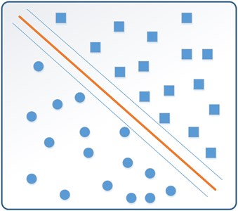
The basic idea of the method is to look for the largest interval separating plane (shows in Fig. 1) in the case of mis-classification which corresponds to the following optimization problem:

5

m i n Φ (w) = \underset{ω, b, ξ}{m i n} (\frac{1}{2} w^{T} w + C \sum_{i = 1}^{N} ξ_{i}),

s . t . {\hat{y}}_{i} [w^{T} x_{i} + b] \geq 1 - ξ_{i}, ξ_{i} \geq 0, i = 1, 2, \dots, N,

where $ξ = (ξ_{1}, ξ_{2}, \dots, ξ_{N})$ , $C > 0$ is a fixed penalty parameter.

Fig. 1The largest interval separating plane of SVM

Eq. (5) can be written as:

6

\underset{\hat{y} \in β}{m i n} \underset{α \in Α}{m a x} G (α, \hat{y}) .

Interchanging the order of $\underset{α \in Α}{m a x}$ and $\underset{\hat{y} \in β}{m i n}$ in Eq. (7), we obtain the proposed WELLSVM:

7

\underset{α \in Α}{m a x} \underset{\hat{y} \in β}{m i n} G (α, \hat{y})

We rewritten the objective of WELLSVM as the following optimization problem:

8

\underset{μ \in Μ}{m i n} \underset{α \in Α}{m a x} \sum_{t : {\hat{y}}_{t} \in β}^{} μ_{t} G (α, \hat{y}),

where $μ$ is the vector of $μ_{t}$ ’s, $Μ$ is the simplex $\{μ |\sum_{t} μ_{t} = 1, μ_{t} \geq 0\}$ , and ${\hat{y}}_{t} \in β$ .

In semi-supervised learning, not all the training labels are known. Let $D_{L} = {\{x_{i}, y_{i}\}}_{i = 1}^{l}$ and $D_{U} = {\{x_{j}\}}_{j = l + 1}^{N}$ be the sets of labeled and unlabeled examples, and $\hat{y} = {[{\hat{y}}_{1}, {\hat{y}}_{2}, \dots, {\hat{y}}_{N}]}^{'}$ is the vector of learned labels on both labeled and unlabeled examples, $y_{L} = {[y_{1}, y_{2}, \dots, y_{l}]}^{'}$ , and ${\hat{y}}_{U} = {[{\hat{y}}_{l + 1}, {\hat{y}}_{l + 2}, \dots, {\hat{y}}_{N}]}^{'}$ [11]. Then the Eq. (5) leads to:

9

m i n Φ (w) = \underset{y \in β}{m i n} \underset{w, ξ}{m i n} (\frac{1}{2} w^{T} w + C_{1} \sum_{i = 1}^{l} ξ_{i} + C_{2} \sum_{i = l + 1}^{N} ξ_{i}),

s . t . {\hat{y}}_{i} [w^{T} x_{i} + b] \geq 1 - ξ_{i}, ξ_{i} \geq 0, i = 1, 2, \dots, N,

where $β = \{\hat{y} = |\hat{y} = [{\hat{y}}_{L}; {\hat{y}}_{U}], {\hat{y}}_{L} = y_{L}, {\hat{y}}_{U} \in {\{\pm 1\}}^{N - 1}\}$ , and $C_{1}$ , $C_{2}$ balance the 2 types of Hinge Loss function:

10

m i n Φ (w) = \underset{μ \in Μ, ξ}{m i n} (\frac{1}{2} \frac{1}{μ_{t}} w^{T} w + C_{1} \sum_{i = 1}^{l} ξ_{i} + C_{2} \sum_{i = l + 1}^{N} ξ_{i}),

s . t . {\hat{y}}_{i} [w^{T} x_{i} + b] \geq 1 - ξ_{i}, ξ_{i} \geq 0, i = 1, 2, \dots, N .

We iterate the following two steps until convergence to solve Eq. (10) by:

1) Fix the mixing coefficients $μ$ of the base kernel matrices.

2) Fix $w_{t}$ ’s and update $μ$ in closed-form.

3. Experimental verification

This section is devoted to show the reliability of the WELLSVM model for fault diagnosis of rolling bearings. Experiment data in different working conditions are chosen to validate the effectiveness of the proposed method.

3.1. Experiment setup

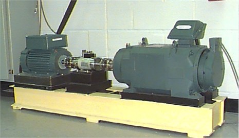
Bearing data from the bearing data center of Case Western Reserve University were used for testing and verification in the experiment. The bearing test-rig contained a 2 horsepower motor which was used as the prime mover to drive a shaft coupled with a bearing housing as shown in Fig. 2. The test-rig included both drive end (DE) and fan end (FE) bearings of 6205-2RS JEM SKF, of which the vibration data were collected by using accelerometers attached to the housing with magnetic bases. Accelerometers were placed at the 3 clock position for both the DE and FE bearings. For data acquisition, digital data was collected at 12,000 samples per second while a sampling rate of 1.2 kHz was used for DE and FE bearing faults.

3.2. Experiment execution

This section we executed the experiment content. Firstly, we did empirical mode decomposition (EMD) to the original signal, the first three IMFs were chosen and then we extracted two different time domain features from each IMF of the used bearing data. We obtained six dimension features from the extracted time domain features. At last, the WELLSVM was employed to classify the four failure mode.

Fig. 2Bearing test-rig for the experiment

Firstly, we clustered inner ring failure, outer ring failure and rolling element failure, and classified them with the normal condition. Then we clustered outer failure and rolling element failure together, and classified them with inner ring failure. After that WELLSVM was used to classify outer ring failure and rolling element failure (shows in Fig. 3). After data processing, for each data set of the mode, 75 % of the examples were randomly chosen for training, and the rest for testing. We investigated the performance of each approach with varying amount of labeled data (namely, 5 %, 10 %, 15 % and 20 % of all the labeled data). The whole setup was repeated 10 times and the average accuracies on the test set are reported in Table 2.

Fig. 3Multi-classification of WELLSVM

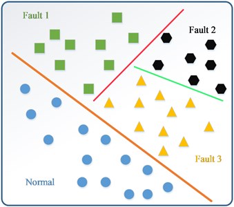
Table 2Average accuracies of fault classification

Classification pattern	Normal with other failure mode	Outer ring with inner ring and rolling element	Inner ring and rolling element
Average accuracies with 5 % labeled	99.24	98.3573	97.728
Average accuracies with 10 % labeled	99.4336	98.872	98.072
Average accuracies with 15 % labeled	99.6608	99.352	98.272
Average accuracies with 20 % labeled	99.6896	99.1093	99.268

3.3. Result and comparison

In Table 2, it is shown that the classification accuracy of 5 %, 10 %, 15 % and 20 % of all the labeled data are all exceeded 95 %, which indicates that the proposed method WELLSVM can separate the normal mode, inner ring failure, outer ring failure and rolling element failure commendably. What’s more, the more labeled examples for training set, the more effective of the result is.

4. Conclusions

In this study, a method of fault diagnosis for rolling bearing is proposed. EMD was utilized as a powerful signal decomposition method for any complicated signal. Because the time domain features can represent the essential characteristics of vibration signals, we extracted the time domain features. At last, WELLSVM was employed as a powerful signal processing method for classification to classify the data of all failure mode which was extracted features from the IMFs. The experiment indicates that WELLSVM can effectively classify fault rolling bearing.

Our future works will focus on the following aspects, firstly, more attempts used WELLSVM will be made to other objects except for rolling bearing. Secondly, we will try to use WELLSVM in another fields except classification to extend the universality of the proposed method.

References

Lou Xinsheng, Loparo Kenneth A. Bearing fault diagnosis based on wavelet transform and fuzzy inference. Mechanical Systems and Signal Processing, Vol. 18, Issue 5, 2004, p. 1077-1095.

Search CrossRef
Kankar P. K., Sharma Satish C., Harsha S. P. Rolling element bearing fault diagnosis using wavelet transform. Neurocomputing, Vol. 74, Issue 10, 2011, p. 1638-1645.

Search CrossRef
Pandya D. H., Upadhyay S. H., Harsha S. P. Fault diagnosis of rolling element bearing with intrinsic mode function of acoustic emission data using APF-KNN. Expert Systems with Applications, Vol. 40, Issue 10, 2013, p. 4137-4145.

Search CrossRef
Fernández-Francos Diego, Martínez-Rego David, Fontenla-Romero Oscar, Alonso-Betanzos Amparo Automatic bearing fault diagnosis based on one-class v-SVM. Computers and Industrial Engineering, Vol. 64, Issue 1, 2013, p. 357-365.

Search CrossRef
Ying Zhao Research on Semi-supervised Support Vector Machine Learning Algorithms. Ph.D. Eng. Theses.

Search CrossRef
Li Yu-Feng, Tsang Ivor W., Kwok James T., Zhou Zhi-Hua Convex and scalable weakly labeled SVMs. Journal of Machine Learning Research, Vol. 14, Issue 1, 2013, p. 2151-2188.

Search CrossRef
Chapelle Olivier, Sindhwani Vikas, Keerthi Sathiya S. Optimization techniques for semi-supervised support vector machines. Journal of Machine Learning Research, Vol. 9, 2008, p. 203-233.

Search CrossRef
Zhao ShuanFeng, Liang Lin, Xu GuangHua, Wang Jing, Zhang WenMing Quantitative diagnosis of a spall-like fault of a rolling element bearing by empirical mode decomposition and the approximate entropy method. Mechanical Systems and Signal Processing, Vol. 40, Issue 1, 2013, p. 154-177.

Search CrossRef
Lee Hong-Hee, Nguyen Ngoc-Tu, Kwon Jeong-Min Bearing diagnosis using time-domain features and decision tree. International Conference on Intelligent Computing, Vol. 4682, 2007, p. 952-960.

Search CrossRef
Bennett Kristin P., Demiriz Ayhan Semi-supervised support vector machine. Proceedings of the Conference on Advances in Neural Information, 1998, p. 368-374.

Search CrossRef
Li Yu-Feng, Tsang Ivor W., Kwok James T., Zhou Zhi-Hua Convex and scalable weakly labeled SVMs. Journal of Machine Learning Research, Vol. 14, Issue 1, 2013, p. 2151-2188.

Search CrossRef

About this article

Received

Accepted

21 August 2015

Published

18 September 2015

SUBJECTS

Fault diagnosis based on vibration signal analysis

Keywords

rolling bearing

fault diagnosis

incomplete labels

weakly labeled support vector machine

Acknowledgements

This study is supported by the National Natural Science Foundation of China (Grant Nos. 61074083, 50705005, and 51105019) and by the Technology Foundation Program of National Defense (Grant No. Z132013B002).

This is an open access article distributed under the Creative Commons Attribution License, which permits unrestricted use, distribution, and reproduction in any medium, provided the original work is properly cited.