Numerical analysis of dynamic characteristics in the ultra-high speed grinding spindle system

Yu, Tianbiao; Wang, Xuezhi; Wang, Wanshan

Journal of Vibroengineering

Browse Journal

Submit article

Published: 15 November 2015

Check for updates

Numerical analysis of dynamic characteristics in the ultra-high speed grinding spindle system

Tianbiao Yu¹

Xuezhi Wang²

Wanshan Wang³

^{1, 2, 3}School of Mechanical Engineering and Automation, Northeastern University, Shenyang, 110819, China

Corresponding Author:

Xuezhi Wang

Cite the article Download PDF

Downloads 1318

Abstract

In this paper, the dynamic characteristics of ultra-high speed grinding spindle system is analyzed by using digital analysis methods. The spindle system is the key components of the machine tool, and its performance directly determines the machining stability and accuracy. Liquid hybrid bearing, with its superior performance has been widely applied to high speed and heavy machine tools. In order to study the spindle system, Fluent software was used to analyze the dynamic characteristics of liquid hybrid bearing. With the increase of the rotational speed, the capacity of liquid hybrid bearing changes significantly, and the relationship between the capacity and rotational is linear in intermediate stage. At the same time, the stiffness and damping of the liquid hybrid bearing has a corresponding increase with the increase of rotational speed. When the rotational speed increase to a certain extent, the dynamic performance of the spindle system will improve. Finally, the concentrated mass method and the finite element analysis method were used to analyze the dynamic characteristics of the spindle system, respectively. The results obtained by the both methods have good consistency, and the critical speed is about 14000 rve/min.

1. Introduction

With the development of processing technology, high-speed machining has become the mainstream of metal cutting. Grinding is not exceptional also. Ultra-high speed grinding technology is a kind of high efficiency, high precision of modern processing technology. Recent progress in ultra-hard abrasives has resulted in the adoption of high wheel speeds to the fixed ultra-high speed grinding process. To achieve this goal, the rotational speed of the spindle must be increased. However, the concomitant problems, such as the working stability and processing accuracy, must be overcome. For ultra-high speed grinding machine, the spindle is a key component, and its dynamic characteristics of spindle system is particularly important [1]. Therefore, it is necessary to study the dynamic characteristics on the spindle system of ultra-high speed grinding machine.

Early studies on spindle systems mainly dealt with static models, calculating stiffness with applied static loads [2]. Many earlier studies attempted to determine the optimal bearing span for spindle design based on these simplified approaches [4]. With the development of processing technology, many researchers have investigated the dynamic aspects of spindles [5-9]. FEM is a commonly used method in the study of dynamic characteristics of the spindle system. W. R. Wang et al. [10] performed a finite-element model (FEM) analysis on a two-bearing spindle, and results shown that internal bearing contact angle variation was more important on the high vibration modes. Chen [11] et al studied the static and dynamic behavior of a shaft supported by hydrostatic bearings by using the finite element method. Rantatalo et al. used FEM and non-contact spindle analyzing lateral vibrations in a milling machine spindle is presented including finite-element modelling, magnetic excitation and inductive displacement measurements of the spindle response [12]. Hong [13] et al. used the finite element method to model the spindle shaft, and analyzed dynamic characteristics of the rotor systems with angular contact ball bearings. In recent years, more and more scholars begin to pay close attention to the nonlinear behavior of bearing bearings. Ding [14] et al. studied an isotropic flexible shaft, acted by nonlinear fluid-induced forces. For the nonlinear rotor system investigated, the synchronous periodic motion loses its stability as the threshold speed is exceeded by the increasing rotating speed.

Start from improving the performance of the machine tool, the dynamic characteristics and the nonlinear behavior of spindle system are both important. However, in the actual process, the root parts determining the spindle performance are bearings. Now ceramic ball hybrid bearings, aerostatic bearing, and liquid hybrid bearing are mainly adopted on ultra-high speed grinding machine due to their ease of maintenance and low cost [2]. Liquid hybrid bearing has some prominent advantages such as larger capacity, longer service life, better dynamic characteristics and higher stiffness. It was used in the ultra-high speed grinding machine of Northeastern University. While there has been a vast amount of research on spindles in the past, few studies focused on the design sensitivity of spindles in terms of bearing configurations [1].

This study provides a systematic analysis of bearing configuration on spindle dynamic. As a result of the liquid hybrid bearing is not traditional, it has shallow oil cavity structure, and is not easy to directly solve nonlinear oil film force by using pure numerical methods. In view of this point, Fluent software was used to analyze the dynamic characteristics of liquid hybrid bearing. On this basis, the dynamic characteristics of spindle system was analyzed. In this paper, CFD simulation and vibration analysis was well combined, and it provides the reference for analyzing the complex bearing support.

2. Mathematical model of a spindle system

2.1. Governing equations

Continuous equation is the mass conservation equation. Any flow must satisfy the law of mass conservation. The law can be stated as: the quality increasing of the fluid micro-unit per unit time is equal to the net mass inflowing in to the micro-body in a unit time. The mass conservation equation can be expressed as follow [15]:

1

\frac{\partial ρ}{\partial t} + \frac{\partial (ρ u)}{\partial x} + \frac{\partial (ρ v)}{\partial y} + \frac{\partial (ρ w)}{\partial z} = 0,

where, $ρ$ is the density of the fluid, $u$ , $v$ , $w$ is the components of the velocity vector in the direction of $x$ , $y$ or $z$ . And for incompressible fluid $\partial ρ / \partial t$ is equal to zero.

N-S Equations is the abbreviation of Navier-Stokes Equation and it is actually momentum conservation equation. The law can be stated as: the change rate of momentum on fluid micro unit per unit time is equal to the sum of external force acting on the micro unit. The law actually is Newton’s second law. According to this law, the momentum conservation equation in the three directions of $x$ , $y$ and $z$ can be derived. Its expressions are as follows [15]:

2

\{\begin{array}{l} \frac{\partial (ρ u)}{\partial t} = ρ f_{x} - \frac{\partial p}{\partial x} + \frac{\partial}{\partial x} \{η [2 \frac{\partial u}{\partial x} - \frac{2}{3} (\frac{\partial u}{\partial x} + \frac{\partial v}{\partial y} + \frac{\partial w}{\partial z})]\} \\ + \frac{\partial}{\partial y} [η (\frac{\partial u}{\partial y} + \frac{\partial v}{\partial x})] + \frac{\partial}{\partial z} [η (\frac{\partial u}{\partial z} + \frac{\partial w}{\partial x})], \\ \frac{\partial (ρ v)}{\partial t} = ρ f_{y} - \frac{\partial p}{\partial y} + \frac{\partial}{\partial y} \{η [2 \frac{\partial v}{\partial y} - \frac{2}{3} (\frac{\partial u}{\partial x} + \frac{\partial v}{\partial y} + \frac{\partial w}{\partial z})]\} \\ + \frac{\partial}{\partial z} [η (\frac{\partial v}{\partial z} + \frac{\partial w}{\partial y})] + \frac{\partial}{\partial x} [η (\frac{\partial v}{\partial x} + \frac{\partial u}{\partial y})], \\ \frac{\partial (ρ w)}{\partial t} = ρ f_{z} - \frac{\partial p}{\partial z} + \frac{\partial}{\partial z} \{η [2 \frac{\partial w}{\partial z} - \frac{2}{3} (\frac{\partial u}{\partial x} + \frac{\partial v}{\partial y} + \frac{\partial w}{\partial z})]\} \\ + \frac{\partial}{\partial x} [η (\frac{\partial w}{\partial x} + \frac{\partial u}{\partial z})] + \frac{\partial}{\partial y} [η (\frac{\partial w}{\partial y} + \frac{\partial v}{\partial z})], \end{array}

where $η$ is the rate of shear deformation, and $ρ f_{i}$ is physical strength acted on the micro unit. When $i$ is $x$ , $y$ or $z$ , it respects the physical strength acted on the micro unit on $x$ , $y$ or $z$ direction.

2.2. Vibration equation

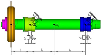
In order to efficiently study spindle system instability, a mathematical model of a rotor-bearing system simulated by four lumped mass points and depicted in Fig. 1 is simplified according to the following assumptions.

(1) The masses of rotor and shaft are lumped at the gravity center of rotor and the equivalent mass in the rotor gravity center, (2) the shaft section is considered massless and rigid. If radial displacements of the rotor center are x and y in the fixed $X$ - $Y$ coordinates and (3) the movements of the rotor in torsional and axial directions are negligible.

And the dynamic equation of the rotor-bearing-seal system can be deduced as follows:

3

M \ddot{q} + (G + C) \dot{q} + K q = F_{e} - F_{g},

where $q$ is the state vector, $F_{e}$ is the eccentric force vector, and $F_{g}$ is the gravity vector. In addition $M$ , $G$ , $C$ , $K$ are respectively mass matrix, gyro matrix , damping matrix and stiffness matrix:

4

q = [x_{1}, θ_{y 1}, x_{2}, θ_{y 2}, x_{3}, θ_{y 3}, x_{4}, θ_{y 4}, y_{1}, θ_{x 1}, y_{2}, θ_{x 2}, y_{3}, θ_{x 3}, y_{4}, θ_{x 4}]^{T},

where $x_{i}$ , $y_{i}$ , $θ_{x i}$ and $θ_{y i}$ ( $i =$ 1, 2, 3, 4) are the displacements in $x$ and $y$ directions and angles of orientation associated with the $x$ and $y$ axes, respectively:

5

M = [\begin{matrix} M_{x} & 0 \\ 0 & M_{y} \end{matrix}], M_{x} = M_{y} = d i a g [m_{1}, J_{d 1}, m_{2}, J_{d 2}, m_{3}, J_{d 3}, m_{4}, J_{d 4}],

6

G = ω J = ω [\begin{matrix} 0 & J_{1} \\ - J_{1}^{T} & 0 \end{matrix}], J_{1} = d i a g [0, J_{p 1}, 0, J_{p 2}, 0, J_{p 3}, 0, J_{p 4}],

where $J_{p i}$ and $J_{d i}$ ( $i =$ 1, 2, 3, 4) are the polar moment of inertia and the diametral moment of inertia, respectively:

7

\{\begin{array}{l} C = C_{1} + C_{2}, \\ C_{1} = α M + β K, \\ C_{2} = d i a g [0,0, c_{x x}, 0,0, 0, c_{x x}, 0,0, 0, c_{y y}, 0,0, 0, c_{y y}, 0], \\ α = \frac{2 (\frac{ξ_{2}}{ω_{2}} - \frac{ξ_{1}}{ω_{1}})}{(\frac{1}{ω_{2}^{2}} - \frac{1}{ω_{1}^{2}})}, \\ β = \frac{2 (ξ_{2} ω_{2} - ξ_{1} ω_{1})}{ω_{2}^{2} - ω_{1}^{2}}, \end{array}

where $ω_{1}$ and $ω_{2}$ are the first and second order natural frequencies (rev/min); $ξ_{1}$ and $ξ_{2}$ are the first and second modal damping ratios; $c_{x x}$ and $c_{y y}$ are the dampings of the left bearing in $x$ and $y$ directions respectively:

8

\{\begin{array}{l} F_{e} = [m_{1} e ω^{2} c o s (ω t), 0,0, 0,0, 0,0, 0, m_{1} e ω^{2} s i n (ω t), 0,0, 0,0, 0,0, 0], \\ F_{g} = [0,0, 0,0, 0,0, 0,0, m_{1} g, 0, m_{2} g, 0, m_{3} g, 0, m_{4} g, 0], \end{array}

where $m_{1} e$ denote eccentricity of unbalance mass of the grinding wheel, and $ω$ is the rotating speeds (rev/min):

9

K = [\begin{matrix} K_{x} & 0 \\ 0 & K_{y} \end{matrix}],

10

K_{x} = [\begin{matrix} k_{11} & k_{12} & k_{13} & k_{14} & 0 & 0 & 0 & 0 \\ k_{12} & k_{22} & k_{23} & k_{24} & 0 & 0 & 0 & 0 \\ k_{13} & k_{23} & k_{33} + k_{x x} & k_{34} & k_{35} & k_{36} & 0 & 0 \\ k_{14} & k_{24} & k_{34} & k_{44} & k_{45} & k_{46} & 0 & 0 \\ 0 & 0 & k_{35} & k_{45} & k_{55} & k_{56} & k_{57} & k_{58} \\ 0 & 0 & k_{36} & k_{46} & k_{56} & k_{66} & k_{67} & k_{68} \\ 0 & 0 & 0 & 0 & k_{57} & k_{67} & k_{77} + k_{x x} & k_{78} \\ 0 & 0 & 0 & 0 & k_{58} & k_{68} & k_{78} & k_{88} \end{matrix}],

11

K_{y} = [\begin{matrix} k_{11} & - k_{12} & k_{13} & - k_{14} & 0 & 0 & 0 & 0 \\ - k_{12} & k_{22} & - k_{23} & k_{24} & 0 & 0 & 0 & 0 \\ k_{13} & - k_{23} & k_{33} + k_{y y} & - k_{34} & k_{35} & - k_{36} & 0 & 0 \\ - k_{14} & k_{24} & - k_{34} & k_{44} & - k_{45} & k_{46} & 0 & 0 \\ 0 & 0 & k_{35} & - k_{45} & k_{55} & - k_{56} & k_{57} & - k_{58} \\ 0 & 0 & - k_{36} & k_{46} & - k_{56} & k_{66} & - k_{67} & k_{68} \\ 0 & 0 & 0 & 0 & k_{57} & - k_{67} & k_{77} + k_{y y} & - k_{78} \\ 0 & 0 & 0 & 0 & - k_{58} & k_{68} & - k_{78} & k_{88} \end{matrix}],

where $k_{x x}$ and $k_{y y}$ denote the stiffnesses of the bearing in $x$ and $y$ directions, respectively. And The matrix elements of $K_{x}$ and $K_{y}$ could be calculated by the following formulas:

\{\begin{array}{l} k_{11} = a_{11}, \\ k_{12} = a_{21}, \\ k_{13} = - a {}_{11}, \\ k_{14} = a_{21}, \end{array} \{\begin{array}{l} k_{22} = l_{1} a_{21} - a_{31}, \\ k_{23} = - a_{21}, \\ k_{24} = a {}_{31}, \end{array} \{\begin{array}{l} k_{33} = a_{11} + a_{12}, \\ k_{34} = - a_{21} + a_{22}, \\ k_{35} = - a {}_{12}, \\ k_{36} = a_{22}, \end{array}

\{\begin{array}{l} k_{44} = l_{1} a_{21} - a_{31} + l_{2} a_{22} - a_{32}, \\ k_{45} = - a_{22}, \\ k_{46} = a {}_{32}, \end{array} \{\begin{array}{l} k_{55} = a_{12} + a_{13}, \\ k_{56} = - a_{22} + a_{23}, \\ k_{57} = - a {}_{13}, \\ k_{58} = a_{23}, \end{array} \{\begin{array}{l} k_{66} = l_{2} a_{22} + l_{3} a_{23} - a_{33}, \\ k_{67} = - a_{23}, \\ k_{68} = a {}_{33}, \end{array}

\{\begin{array}{l} k_{77} = a_{13}, \\ k_{78} = - a_{23}, \\ k_{88} = l_{3} a_{23} - a_{33}, \end{array} \{\begin{array}{l} a_{1 i} = \frac{12 E I}{{l_{i}}^{3}}, \\ a_{2 i} = \frac{1}{2} l_{i} a_{1 i}, \\ a_{3 i} = \frac{1}{6} {l_{i}}^{2} a_{1 i}, i = 1, 2, 3 . \end{array}

In addition $E$ , $I$ and $l_{i}$ are the Young’s modulus of elasticity, the area moment of inertia and the distance between every two adjacent lumped mass points respectively.

Fig. 1The diagram of spindle system

3. Result discussion

3.1. Calculating kinetic parameters of bearing

3.1.1. Calculating oil film force

Before the analysis, the oil film model should be established firstly. The structure diagram of liquid hybrid bearing is shown as Fig. 2(a), and the basic structural parameters is shown as Table 1. On this basic the calculating model of oil film can be established. Firstly, the finite element model of the film was built by using gambit, and then the model was divided into the grid model in this paper. The grid is divided into more than 670,000 hexahedral grid cells. The entrance is the inlet with five dopers, which is set as pressure inlet. The exit is the end face of the bearing, which is set as pressure exit. The inside surface and the outside surface of the film are set as wall boundary. Three-dimensional model of oil is shown in Fig. 2(b).

Fig. 2Entity of liquid hybrid bearing and three-dimensional model of film

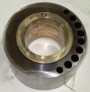
a) Entity of liquid hybrid bearing

b) Three-dimensional model of oil film

Table 1Structure parameters of liquid hybrid bearing

Parameter name	Code	Value
Diameter of liquid hybrid bearing	$D$	80.0 mm
Width of liquid hybrid bearing	$B$	80.0 mm
Average thickness of oil film	$h_{0}$	0.03 mm
Depth of oil cavity	$c$	0.25 mm
Width of oil cavity	$b$	36.0 mm
Circumferential central Angle of oil cavity	$δ$	52°
Diameter of orifice	$d_{c}$	1.0 mm
Depth of orifice	$h_{c}$	3.0 mm
Diameter of equalizing oil cavity	$d_{r}$	2.5 mm
Depth of equalizing oil cavity	$h_{r}$	3.0 mm

This paper adopted the Fluent software to solve the flow field of the liquid hybrid bearing. And an implicit stationary model was adopted to calculate, and the physical model is set as turbulent flow. The steady state model was used to calculate the flow of liquid hybrid bearing. The flow media was set as No. 2 main shaft oil. It parameters such as density $ρ =$ 810 kg/m³, specific heat capacity $C_{p} =$ 2000 J/kg K and heat conductivity coefficient $λ =$ 0.37 w/m K. In addition dynamic viscosity $μ$ of No. 2 main shaft oil was considered the influence of temperature, and its dynamic viscosity at different temperature was calculated by Eq. (12) [16]:

12

μ_{T} = μ_{o} \times e x p [159.5578737 (\frac{1}{T + 95} - 0.001140089) l n \frac{μ_{40}}{μ_{o}}] .

In this equation, dynamic viscosity of No. 2 main shaft oil at $T$ °C could be calculated based on that of 40 °C , $μ_{o} =$ 0.18×10^-3 kg/m∙s and $μ_{40} =$ 2.23×10^-3 kg/m∙s. After calculating, the dynamic viscosity of No. 2 main shaft oil is shown in Table 2.

After setting essential parameter, the initial states of calculation model should be set, and they are oil pressure, oil temperature, spindle speed and eccentricity of the liquid hybrid bearing. Oil pressure $P_{i}$ changes from 1 to 7 MPa, oil temperature $T_{i}$ changes from 293 K to 323 K, spindle speed $n$ changes from 0 to 20000 rve/min and eccentricity ratio $ζ$ changes from 0.2 to 0.5. On these basic, oil film temperature of different working condition were obtained through the simulation, and the results were shown in Fig. 3. As a result of the existence of eccentric, the pressure balance of the oil film is broke. Meanwhile the high pressure area appears and it mainly concentrates in the eccentric position. The pressure of oil cavity is higher than that of oil sealing face. With the increase of rotational speed, dynamic pressure effect becomes increasingly obvious, and the high pressure area gradual expands along the bearing running direction.

Table 2Dynamic viscosity at different temperatures

Temperature $T$ (°C)	20	30	40	50	60	70	80
Dynamic viscosity $μ_{T}$ (10^-3 kg/m∙s)	3.74	2.83	2.23	1.82	1.52	1.30	1.13

Fig. 3Oil film pressure distribution

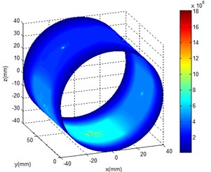
a) $ω =$ 0 rve/min

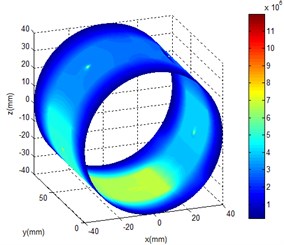
b) $ω =$ 5000 rve/min

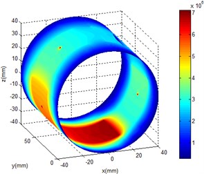
c) $ω =$ 10000 rve/min

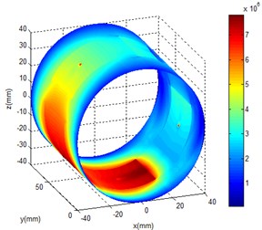
d) $ω =$ 20000 rve/min

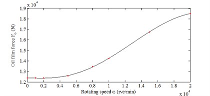
The capacity is the foundation for studying the dynamic characteristics of liquid hybrid bearing. So it is necessary to calculate the dynamic bearing capacity of the liquid hybrid bearing. When eccentricity ratio of liquid hybrid bearing, the temperature and the pressure of oil supply are constant. With the increase of rotational speed, the capacity of liquid hybrid bearing changes significantly. The change of capacity can be divided into three stages. When the rotational speed is less than 5000 rve/min, the capacity remains basically unchanged. When the rotational speed is at the stage of 5000-15000 rve/min, the relationship between the capacity and rotational speed is linear. When the rotational speed is more than 15000 rve/min, with the increase of rotational speed, the growth of capacity is slowing down. The result is shown in Fig. 4. The main reason is that the effect of dynamic pressure is not evident comparing with static pressure at a low rotational speed. At the middle rotational speed stage, when the rotational speed reaches a certain value, the effect of the dynamic pressure gradually highlights. And with the further increase of rotational speed, the growth of capacity is slowing down. When the liquid hybrid bearing works in a high rotational speed, the oil temperature will rise quickly and the oil viscosity reduce at the same time. In a sense, as the rotational speed increasing, the capacity of liquid hybrid bearing will not have been rising. When the rotational speed reaches a certain value, the capacity may decline. Even failure may occur.

Fig. 4Dynamical capacity of liquid hybrid bearing

3.1.2. Calculating oil film stiffness and damping

The joint is an important part of a rotor system. As the stiffness and irreversible deformation due to the contact fatigue of the structure have an obvious impact on the rotor dynamics and imbalance response, the stiffness and contact state must be considered in the rotor joint dynamic design. In this section, impact of geometrical parameter and external load upon the joint are studied by numerical method.

The stiffness of structures can be measured from global and local perspectives. From a global point of view, the stiffness is reflected by the flexural deformation under the external bend load; from a local point of view, the stiffness is reflected by the geometry of shaft section and material properties, which is the sectional flexural stiffness. Due to the existence of the contact surface of joints, the shaft with the joint is a non-continuous body. The stiffness related to the joint could not be described by sectional flexural stiffness from the local perspective.

Consider the hydrodynamic bearing described in Fig. 2. Using the small perturbation method, the increment of fluid-film stiffness and damping components can be described as follows:

13

\{\begin{array}{l} k_{x x} = \frac{\partial F_{x}}{\partial x} = l i m (\frac{Δ F_{x}}{Δ x}), \\ k_{y y} = \frac{\partial F_{y}}{\partial y} = l i m (\frac{Δ F_{y}}{Δ y}), \end{array}

14

\{\begin{array}{l} c_{y y} = \frac{\partial F_{x}}{\partial^{2} x} = l i m (\frac{Δ F_{x}}{Δ \dot{x}}), \\ c_{y y} = \frac{\partial F_{y}}{\partial^{2} y} = l i m (\frac{Δ F_{y}}{Δ \dot{y}}), \end{array}

where $Δ F_{x}$ and $Δ F_{y}$ represent the increment of oil film force in the $X$ direction and $Y$ direction; and $Δ x$ , $Δ y$ , $Δ \dot{x}$ and $Δ \dot{y}$ represent the perturbation of displacements and velocities in the $X$ direction and $Y$ direction, respectively.

By giving small perturbations of displacement either in the $X$ direction or $Y$ direction, the stiffness coefficients can be obtained by differentiating the resultant fluid film force components on the displacements of perturbation. In standard lubrication programs, the dimensionless perturbation of displacements $Δ x / h_{0}$ , $Δ y / h_{0}$ is usually between 0.01 and 0.005 [18]. For better comparison, two dimensionless perturbations are used: 0.01 and 0.005 for selected CFD results. In order to calculate the damping coefficients, a special capability in FLUENT, called “Moving Grid”, has been employed. The bearing surface and journal surface are specified as “Frozen” nodes and “Moved” nodes, respectively. To match with the practice in standard codes, the dimensionless perturbations of velocity used in this study are $Δ \dot{x} / h_{0} =$ 0.005 and $Δ \dot{y} / h_{0} =$ 0.005. The rigidity and the damping of oil film under different rotational speed were obtained by calculating, and the results were shown in Table 3. In the range of 0-20000 rve/min, with the increase of rotational speed, the stiffness and the damping of the bearing increases constantly, and the change in the low speed region is more obvious.

Table 3Oil film stiffness and damping at different rotational speeds

$ω$ (10³ rev/min)	$k_{x x}$ (10⁸ N/m)	$k_{y y}$ (10⁸ N/m)	$c_{x x}$ (10⁵ N⋅s/m)	$c_{y y}$ (10⁵ N⋅s/m)
0	5.31	3.44	1.69	1.71
2	5.92	3.87	1.84	1.87
5	6.68	4.36	2.11	2.16
8	7.58	5.01	2.34	2.41
10	8.03	5.42	2.57	2.69
15	9.01	6.27	2.81	2.86
20	9.44	6.65	3.04	3.11

3.2. Vibration responses

The natural frequencies of a rotor-bearing system are determined by the mass and stiffness of the rotor, and the stiffness of supporting bars. First, a transfer matrix method is used to calculate these undamped natural frequencies. The spindle system is simplified as for lumped masses and three massless elastic beams, as shown in Fig. 1. Values of these masses and beams are shown in Table 4. For the model with retainer spring, the system can be considered as pinned at one end and supported by a spring at the position of front-end of spindle. The stiffness of this spring is shown in Table 3, and the transfer matrix calculation gives the first undamped natural frequency at 217.55 Hz and the second at 661.33 Hz.

Table 4Model parameters of the spindle system

Parameters	Value
$m_{1}$ , $m_{2}$ , $m_{3}$ , $m_{4}$ (kg)	22.92, 10.23, 15.24, 8.39
$J_{p 1}$ , $J_{d 1}$ (10^-5 kg⋅m²)	2.65, 1.38
$J_{p 2}$ , $J_{d 2}$ (10^-5 kg⋅m²)	0.65, 0.37
$J_{p 3}$ , $J_{d 3}$ (10^-5 kg⋅m²）	1.78, 0.89
$J_{p 4}$ , $J_{d 4}$ (10^-5 kg⋅m²)	0.52, 0.26
$ξ_{1}$ , $ξ_{2}$	0.04, 0.02

Rotational speed is a key parameter in affecting the dynamic characteristics of the whole rotational system. With the increase of rotational speed, the stiffness will be dramatically improved. When the rotational speed reaches 20000 rve/min, the stiffness will reach 9.44×10⁸ N/m, and it is 1.78 times of the initial value. Consequently, the stiffness matrix becomes nonlinear, and the detailed stiffness values are shown in Table 3. Since the combined mass and stiffness matrices are to be inverted only once prior to the iteration loop, the computational rigor is significantly relieved. The equation of motion and its solution by the modified Newmark’s direct integration method as described above are applied in this study to the spindle system.

Fig. 5 shows the time response of left axis (center of No. 2) under the different rotational speed. It shows that the dynamic of rotational speed inputs is also irregular at this time. With the increase of rotational speed, the amplitude and the vibration are more and more intense, but it's not hard to see, the movement of the axis is still the periodic.

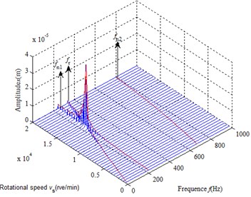
In order to deeply understand the dynamic character of the spindle system of the ultra-high speed grinder, the frequency response analysis was carried out on the axis of motion. The change of dynamic characteristics of rotating machinery is well achieved through stiffness adjustment. Fig. 6 shows the waterfall diagram of damper vibration for this case. It can be seen from the waterfall diagram that the rotating speed from 0 to 13000 rev/min the vibration is essentially synchronous. When the rotating speed $ω$ approaches about the first natural frequency (about 14000 rev/min), a severe vibration appears. In addition, first order vibration is more severe than second order vibration.

Fig. 5Vibration waveforms

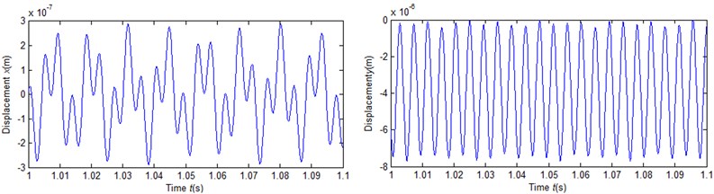
a) $ω =$ 5000 rve/min

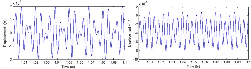
b) $ω =$ 10000 rve/min

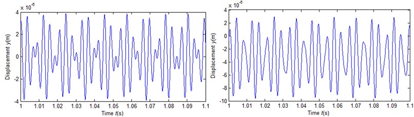
c) $ω =$ 20000 rve/min

Fig. 6Waterfall diagram of damper vibration

3.3. Finite element analysis

Lumped mass method is a simplified method in dynamics analysis. In order to verify the mathematical model of the spindle system, the finite element method is used in the section. Ansys11.0 is used for modal analysis to the spindle system. And the entity model is divided into 5738 nodes. In the FEM model, Solid 45 is used, which has 8 nodes and 6 freedoms. Combine14 is used to simulate the liquid hybrid bearing and axial freedom of the system is limited. And the Stiffness and damping are still using the results in Table 2. The materials of spindle and grinding wheel’s matrix are both 40 Gr, and material properties are shown in Table 5. The finite element model of spindle system is shown in Fig. 7. By the calculation, the vibration model of the spindle system and the modal frequency were obtained, and the results are respectively shown in Fig. 8 and Fig. 9.

Table 5Material properties

Material	Density $ρ_{40 G r}$ (kg/m³)	Elastic modulus $E_{40 G r}$ (N/m²)	Poisson’s ratio $ε$
40 Gr	7.85×10³	2.06×10¹¹	0.3

Fig. 7The finite element model of spindle system

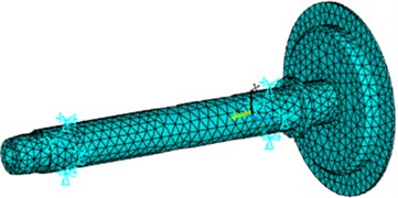
Fig. 8 shows the first order is cantilever oscillating and the second order is spindle bending vibration. In the first order model, the grinding wheel swings. In general, the cantilever oscillating rarely appears in the first order modal. It is mainly attributed to size and quality of the grinding wheel. In the second order model, the bending deflection occurs in the middle of the spindle.

Fig. 8The modal shape of the spindle system

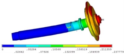
a) First order modal shape

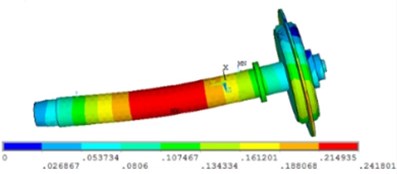
b) Second order modal shape

Fig. 9The results of finite element analysis

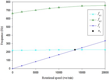
Fig. 9 shows that rotational speed has a certain influence on modal frequency. Where $f_{n 1}$ is the first order frequency, $f_{n 2}$ is the second order frequency, $f_{r}$ is the rotation frequency and $n_{1}$ is the critical speed of rotation. And with the increase of rotational speed the modal frequency gradually increases. This is mainly due to the stiffness increased. The influence of the rotational speed on the second order frequency is more significant. Using graphical method, the critical speed of rotation is obtained, and its value is about 13500 rve/min. It is close to the results obtained by Lumped mass method.

4. Conclusion

Dynamic characteristics of variable stiffness spindle system is discussed in this paper. It focuses on how the rotational speed affect the stiffness of liquid hybrid bearing and the dynamic characteristics of spindle system. These following conclusions are obtained:

1) The method combining CFD simulation with dynamic analysis is an effective method in analyzing the dynamic characteristics of the spindle system. In addition, the difficulty could be reduced by using the method to some extent.

2) The emergence of the imbalance of oil film force is due to the existence of the eccentric. It is increased with the rotational speed growth, and leads to the increase of film damping and stiffness. This feature is more noticeable at medium speed for liquid hybrid bearing operation stage performance. At this stage, the relationship between the capacity of the liquid hybrid bearing and rotational speed is approximate linear. But with the further increase of rotational speed, the growth of capacity is slowing down.

3) The stiffness has significant influence on the dynamic characteristics, with the increase of rotational speed, the stiffness increases slowly, and natural frequency of the system gradually rises. Therefore, the increasing of the first critical speed resulted from the increasing of the stiffness. Based on the characteristics of the liquid hybrid bearing, it is necessary to considering the variable stiffness characteristics in dynamics analyzing the spindle system of the ultra-high speed grinder.

References

Cao Y. Z., Yusuf A. A general method for the modeling of spindle-bearing systems. Journal of Mechanical Design, Vol. 126, Issue 11, 2004, p. 1089-1104.

Search CrossRef
Li H. Q., Yung C. S. Analysis of bearing configuration eﬀects on high speed spindles using an integrated dynamic thermo-mechanical spindle model. International Journal of Machine Tools and Manufacture, Vol. 44, 2004, p. 347-364.

Search CrossRef
Li C. H., Cai G. Q., Ding Y. C., et al. Key technology and application for super-high speed grinding machining. Sciencepaper Online, Vol. 3, Issue 8, 2008, p. 618-623.

Search CrossRef
Li H., Shin Y. C. Integrated dynamic thermo-mechanical modeling of high speed spindles, part 1: model development. Journal of Manufacturing Science and Engineering, Vol. 126, Issue 1, 2004, p. 148-158.

Search CrossRef
Lin C. W., Tu J. F. Model-based design of motorized spindle systems to improve dynamic performance at high speeds. Journal of Manufacturing Processes, Vol. 9, Issue 2, 2007, p. 94-108.

Search CrossRef
Mane I., Gagnol V., Bouzgarrou B. C., et al. Stability-based spindle speed control during flexible workpiece high-speed milling. International Journal of Machine Tools and Manufacture, Vol. 48, Issue 2, 2008, p. 184-194.

Search CrossRef
Faassen R. P. H., Wouw N. V. D., Oosterling J. A. J., et al. Prediction of regenerative chatter by modelling and analysis of high-speed milling. International Journal of Machine Tools and Manufacture, Vol. 43, Issue 14, 2003, p. 1437-1446.

Search CrossRef
Gagnol V., Bouzgarrou B. C., Ray P., et al. Model-based chatter stability prediction for high-speed spindles. International Journal of Machine Tools and Manufacture, Vol. 47, Issue 7, 2007, p. 1176-1186.

Search CrossRef
Luo Xiaoying, Tang Jinyuan Effect of structure parameters on dynamic properties of spindle system. Chinese Journal of Mechanical Engineering, Vol. 43, Issue 3, 2007, p. 128-134, (in Chinese).

Search CrossRef
Wang W. R., Chang C. N. Dynamic analysis and design of a machine tool spindle-bearing system, Journal of Vibration and Acoustics, Vol. 116, 1994, p. 280-285.

Search CrossRef
Chen D. J., Fan J. W., Zhang F. H. Dynamic and static characteristics of a hydrostatic spindle for machine tools. Journal of Manufacturing Systems, Vol. 31, Issue 11, 2010, p. 26-33.

Search CrossRef
Rantatalo M., Aidanpää J. O., Göransson B., et al. Milling machine spindle analysis using FEM and non-contact spindle excitation and response measurement. International Journal of Machine Tools and Manufacture, Vol. 47, Issue 7, 2007, p. 1034-1045.

Search CrossRef
Hong S. W., Kang J. O., Shin Y. C. Dynamic analysis of rotor systems with angular contact ball bearings subject to axial and radial loads. International Journal of the Korean Society of Precision Engineering, Vol. 3, Issue 2, 2002, p. 61-71.

Search CrossRef
Ding Q.,·Zhang K. P. Order reduction and nonlinear behaviors of a continuous rotor system. Nonlinear Dynamics, Vol. 67, 2012, p. 251-262.

Search CrossRef
Han Zhanzhong, Wang Jing, Lan Xiaoping FLUENT – Fluid Simulation Calculating Examples and Engineering Application. Beijing Institute of Technology Press, Beijing, 2010, p. 14-16, (in Chinese).

Search CrossRef
Jiang Jihai, Zhang Dongquan Viscosity-temperature equation of reference temperature t = 40°C. Machine Tool and Hydraulics, Issue 5, 1997, p. 14, (in Chinese).

Search CrossRef
Li X. T., Han Z. N. Rotator critical rotational speed and modal analysis based on ANSYS. Mechanical Management and Development, Vol. 25, Issue 3, 2010, p. 184-185.

Search CrossRef
Guo Z. L., Hirano T., Kirk R. G. Application of CFD analysis for rotating machinery – part 1: hydrodynamic, hydrostatic bearings and squeeze film damper. Journal of Engineering for Gas Turbines and Power, Vol. 127, 2005, p. 445-451.

Search CrossRef

About this article

Received

10 July 2015

Accepted

26 September 2015

Published

15 November 2015

SUBJECTS

Mechanical vibrations and applications

Keywords

ultra-high speed grinding

spindle system

liquid hybrid bearing

dynamic characteristics

stiffness

critical speed

Acknowledgements

The authors acknowledge the support from the National Natural Science Foundation of China (No. 51275084) and the Key Laboratory Foundation of Liaoning Province of China (No. LS2010066).

This is an open access article distributed under the Creative Commons Attribution License, which permits unrestricted use, distribution, and reproduction in any medium, provided the original work is properly cited.