Study of synchronization for a rotor-pendulum system with Poincare method

Fang, Pan; Hou, Yongjun; Nan, Yanghai; Yu, Le

Journal of Vibroengineering

Browse Journal

Submit article

Published: 15 August 2015

Check for updates

Study of synchronization for a rotor-pendulum system with Poincare method

Pan Fang¹

Yongjun Hou²

Yanghai Nan³

Le Yu⁴

^{1, 2, 4}School of Mechanical Engineering, Southwest Petroleum University, Chengdu, China

³Department of Mechanical Engineering and Robotics, Universite Libre de Bruxelles, Brussel, Belgium

Corresponding Author:

Yongjun Hou

Cite the article Download PDF

Downloads 1127

Abstract

A simplified model of the system of unbalanced rotors coupled with pendulum rod is examined. The model consists of two counter-rotating rotors, a rigid pendulum rod and a rigid vibrating body, which is horizontally connected to a fixed support by means of springs. The synchronous state of the system, i.e. synphase and antiphase synchronization of the rotors, is studied by means of the Poincare method. Moreover, the assessment of the synchronous state is converted to find a solution that should satisfy a balanced function and a stability function of the system. However, frequency ratios and installation angular are included in the two functions. It is demonstrated that the spring stiffness and the installation angular have a large influence on the existence and stability of the synchronization state in the coupling system. Finally, computer simulations are preformed to verify the theoretical computations.

1. Introduction

The word “synchronization” is often encountered in both science and daily life. Our surroundings are full of synchronization phenomenon, which is considered as an adjustment of rhythms of oscillating objects due to their internal weak couplings [1]. For examples: violinists play in unison; insects in a population emit acoustic or light pulses with a common rate; birds in a flock flap their wings simultaneously; the heart of a rapidly galloping horse contracts once per locomotory cycle, etc. [2]. Synchronization phenomenon in large populations of interacting elements are the subjects of intense research efforts in physical, biological, chemical and social system, however, the most representatives are synchronization of complex systems [3-5], coupled with pendula or mechanical rotors in recent years. For the synchronization of pendula, in the particular case of the Huygens’ clocks system, the remarkable feature reported by Huygens in 1665 is that pendulum clocks synchronize in antiphase. Nowadays the synchronized limit behavior of Huygens’ clocks, synphase and antiphase synchronization of the pendula, is studied considering the difference values of spring stiffness [6, 7]. Meanwhile, the synchronization of derivatizations of Huygens’ clocks, including two coupled double pendula [8], pendulum coupled by an elastic force [9] and pendula connected by linear springs [10], have been attracting many scholars’ attention. For the synchronization of rotors, I. I. Blekhman [1] proposed the Poincare method for the synchronization state and stabilty and by now this method is widely used in engineering. Based on Blekhman’s method, many scientists have been developing the other methods to analyze the synchronization of the rotors. Wen et al. [11] developed the average method to investigate synchronization and stability of multiple rotors in after-resonance. Zhang et al. [12, 13] described the average method of modified small parameters, which immensely simplify the process for solving the problems of synchronization of the rotors. Sperling et al. [14] presented analytical and numerical investigation of a two-plane automatic balancing device, for equilibration of rigid-rotor unbalance. Balthazar [15, 16] examined self-synchronization of four non-ideal exciters in non-linear vibration system via numerical simulations. Djanan A. A. N. [17] explored the condition, for which three motors working on a same plate, can enter into synchronization with the phase difference depending on the physical characteristics of the motors and the plate.

The above-mentioned researches are mainly synchronization of the pendula or the rotors; however, the synchronization of the rotors coupled with pendula is less reported. Recently, we have purposed that synchronization of two homodromy rotors coupled with a pendulum rod in an after-resonant system, but the influence of the variation of the spring stiffness on the synchronous state of the rotors is less considered. This paper is a continuation of our published literature by means of the Poincare method, building on the original work of Blekhman. Here, we consider the model of a two counter-rotating rotors coupled with a rigid pendulum rod through a torsion spring, and the vibrating body is horizontally connected to a fixed support by means of springs. It is demonstrated that the spring stiffness and the installation angular of the pendulum have a large influence on the existence and stability of the synchronization state in the coupling system.

This paper is organized as follows. Section 2 describes the strategy and considered model. In Section 3, we employ the Laplace transform method to calculate the value of the coupling coefficients. In Section 4, we derive the synchronization equation and the synchronization criterion of the system. In Section 5, we compare and analyze the values of the stable phase difference with theoretical computations and the computer simulations. Finally, we summarize our results in Section 6.

2. Strategy and model

2.1. Strategy

Consider the dynamic equation of a rotation system:

1

J_{s} {\ddot{φ}}_{s} = μ Φ_{s} (φ_{s}, \ddot{x}), (s = 1, \dots, k),

\ddot{x} + 2 ω_{x} ξ_{x} \dot{x} + ω_{x}^{2} x = \sum_{j = 1}^{k} F_{j} (ω t, α_{1}, \dots, α_{k}) + μ F_{k + 1} (ω t, α_{1}, \dots, α_{k}),

where $μ Φ_{s} = M_{e s} - R_{e s}$ , $μ$ is a small parameter, $J_{s}$ is the rotational inertia of the $s$ th induction motors, $R_{e s}$ is the mechanical damping torque of the motors, $ξ_{x}$ is the damping ratio of the system in the $x$ -direction, $ω_{x}$ is natural frequency of the system in $x$ -direction. $ω$ and $φ_{s}$ are mechanical velocity and phase angular of the $s$ thunbalanced rotor, respectively.

Based on the Eq. (1), the following sequence of analysis for vibration system employing synchronizing rotors can be formulated:

1) Steady forced vibrations with $T = 2 π / ω$ are determined by:

2

x = x (ω t, α_{1}, \dots, α_{k}),

the supporting body or supporting system of bodies (i.e., from the second formula of Eq. (2) considering $μ = 0$ ) when rotors are uniformly rotating with initial phase $α_{1}$ ,…, $α_{k}$ , i.e.:

3

φ_{s} = φ_{s}^{0} = (ω t + α_{s}) .

2) Above-mentioned Eq. (3) may correspond only to such values of constants $α_{1}$ ,…, $α_{k}$ , which satisfy:

4

P_{s} (α_{1}, \dots, α_{k}) = μ ⟨Φ_{s} (φ_{s}, \ddot{x})⟩ = 0,

where the angle brackets $⟨*⟩$ show the average within $T$ , i.e.:

5

⟨*⟩ = \frac{1}{T} \int_{0}^{T} * d t,

where symbol $*$ represents a function related to time $t$ [1].

3) If a certain set of constants $α_{1} = α_{1}^{*}, \dots, α_{k} = α_{k}^{*}$ , which satisfy Eq. (4), real parts of all roots $χ$ of the $k$ th order algebraic equation:

6

|\begin{matrix} \frac{\partial (P_{1} - P_{k})}{\partial α_{1}} - χ & \frac{\partial (P_{1} - P_{k})}{\partial α_{2}} & \dots & \frac{\partial (P_{1} - P_{k})}{\partial α_{k - 1}} \\ \frac{\partial (P_{2} - P_{k})}{\partial α_{1}} & \frac{\partial (P_{2} - P_{k})}{\partial α_{2}} - χ & \dots & \frac{\partial (P_{2} - P_{k})}{\partial α_{k - 1}} \\ \dots & \dots & \dots & \dots \\ \frac{\partial (P_{k - 1} - P_{k})}{\partial α_{1}} & \frac{\partial (P_{k - 1} - P_{k})}{\partial α_{2}} & \dots & \frac{\partial (P_{k - 1} - P_{k})}{\partial α_{k - 1}} - χ \end{matrix}| = 0,

are negative, then at sufficiently small $μ$ this set of constant is indeed correlated with the unique, analytical relative to $μ$ , asymptotically stale periodic solution of Eq. (1). This solution changes into the fundamental solution (Eq. (4)) at $μ = 0$ . If the real part of at least one root of Eq. (6) is positive, then the corresponding solution is unstable. With purely imaginary zero roots, an additional analysis is requires in general case [1].

2.2. Model

A simplified rotor-pendulum system depicted in Fig. 1 is considered. This model consists of a rigid vibrating body of mass $m_{0}$ [Kg] elastically supported via a linear spring with stiffness $k_{x}$ [N/m] and a linear viscous damper with damping constant $f_{x}$ [Ns/m]. Unbalanced rotor $i$ is modelled by a point mass $m_{i}$ [Kg] (for $i =$ 1, 2) attached at the end of a massless rod of length $r$ [m]. One of the unbalanced rotors in the system is directly mounted on the vibrating body, and the other is fixed at the end of a pendulum rod, connected with the vibro-platform by a linear torque spring with stiffness $k_{φ}$ [N/rad] and a linear viscous damper with damping constant $f_{φ}$ [Nm/(rad/s)]. The rotation angle of rotor $i$ is denoted by $φ_{i} \in S^{1}$ (for $i =$ 1, 2) in [rad]; the oscillating angle of the pendulum rod is denoted by $φ_{3} \in S^{1}$ in [rad]; the installation angle of the pendulum rod is expressed by $β \in S^{1}$ in [rad]; $x$ is the horizontal displacement of the vibro-platform in [m]; and $M_{e i}$ represents the electromagnetic torque of the induction motors in [N/m].

Then expressions for kinetic and potential energy of the system can be written as follows:

7

T = \frac{1}{2} m_{0} {\dot{x}}^{2} + \frac{1}{2} m_{1} [(\dot{x} + r {\dot{φ}}_{1} s i n φ_{1})^{2} + (r {\dot{φ}}_{1} c o s φ_{1})^{2}]

+ \frac{1}{2} m_{2} [(\dot{x} - r {\dot{φ}}_{2} s i n φ_{2} - l {\dot{φ}}_{3} s i n (β + φ_{3}))^{2} + (r {\dot{φ}}_{2} c o s φ_{2} + l {\dot{φ}}_{3} c o s (β + φ_{3}))^{2}]

+ \frac{1}{2} m_{3} [(\dot{x} - l {\dot{φ}}_{3} s i n (β + φ_{3}))^{2} + (l {\dot{φ}}_{3} c o s (β + φ_{3}))^{2}] + \frac{1}{2} \sum_{i = 1}^{3} J_{i} {\dot{φ}}_{i}^{2} .

Moreover, the potential energy of the system can be given as follows:

8

V = \frac{1}{2} k_{x} x^{2} + \frac{1}{2} k_{φ} φ_{3}^{2} .

In addition, the viscous dissipation function of the system can be expressed in form:

9

D = \frac{1}{2} f_{x} {\dot{x}}^{2} + \frac{1}{2} f_{1} {\dot{φ}}_{1}^{2} + \frac{1}{2} f_{2} {\dot{φ}}_{2}^{2} + \frac{1}{2} f_{3} {\dot{φ}}_{3}^{2} .

The dynamics equation of the system is established by using the Lagrange’s equation:

10

\frac{d}{d t} \frac{\partial T}{\partial {\dot{q}}_{i}} - \frac{\partial (T - V)}{\partial q_{i}} + \frac{\partial D}{\partial {\dot{q}}_{i}} = Q_{i} .

Fig. 1Simplified model

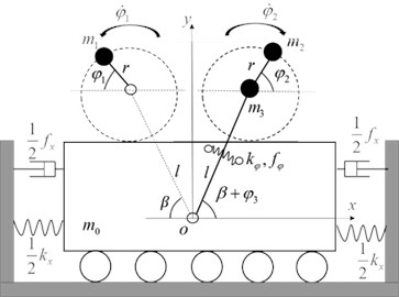
If $q = {x, φ_{1}, φ_{2}, φ_{3}}$ is chosen as the generalized coordinates, the generalized force are $Q_{x} = Q_{φ_{3}} = 0$ , $Q_{φ_{1}} = M_{e 1} - R_{e 1}$ , $Q_{φ_{2}} = M_{e 2} - R_{e 2}$ . Assuming $m_{1} ≪ m_{0}$ and $m_{2} ≪ m_{0}$ in the system, the inertia coupling from asymmetry of the rotors and the pendulum rod can be neglected. Considering $\sum_{k = 0}^{3} m_{k} = M,$ $m_{1} = m_{2} = m,$ $J_{1} + m_{1} r^{2} \approx m_{1} r^{2},$ $J_{2} + m_{2} r^{2} \approx m_{2} r^{2},$ $J_{3} + m_{2} l^{2} + m_{3} l^{2} \approx m_{2} l^{2} + m_{3} l^{2}$ and substituting Eqs. (7), (8) and (9) into (10), we can obtain the dynamic equation of the vibration system:

11

\{\begin{array}{l} M \ddot{x} + f_{x} \dot{x} + k_{x} x = (\begin{matrix} - m r ({\ddot{φ}}_{1} s i n φ_{1} + {\dot{φ}}_{1}^{2} c o s φ_{1}) + m r ({\ddot{φ}}_{2} s i n φ_{2} + {\dot{φ}}_{2}^{2} c o s φ_{2}) \\ + (m l + m_{3} l) [{\ddot{φ}}_{3} s i n β + {\dot{φ}}_{3}^{2} c o s β] \end{matrix}), \\ m r^{2} {\ddot{φ}}_{1} = M_{e 1} - R_{e 1} - m r \ddot{x} s i n φ_{1}, \\ m r^{2} {\ddot{φ}}_{2} = M_{e 2} - R_{e 2} + m r [\ddot{x} s i n φ_{2} - l {\ddot{φ}}_{3} c o s (β - φ_{2}) + l {\dot{φ}}_{3}^{2} s i n (β - φ_{2})], \\ (m l^{2} + m_{3} l^{2}) {\ddot{φ}}_{3} + f_{φ} {\dot{φ}}_{3} + k_{φ} φ_{3} = (\begin{matrix} (m l + m_{3} l) \ddot{x} s i n β \\ - m r l [{\ddot{φ}}_{2} \cos (φ_{2} - β) + {\dot{φ}}_{2}^{2} \sin (φ_{2} - β)] \end{matrix}) . \end{array}

Considering the solution of the problem by the Poincare method (i.e., based on the fundamental Eq. (1)), we will introducing the small parameter $μ$ into Eq. (11), thus presenting it in the form:

12

\{\begin{array}{l} M \ddot{x} + k_{x} x = (\begin{matrix} - m r ({\ddot{φ}}_{1} s i n φ_{1} + {\dot{φ}}_{1}^{2} c o s φ_{1}) + m r ({\ddot{φ}}_{2} s i n φ_{2} + {\dot{φ}}_{2}^{2} c o s φ_{2}) \\ + (m l + m_{3} l) {\ddot{φ}}_{3} s i n β + μ [(m l + m_{3} l) {\dot{φ}}_{3}^{2} c o s β] - μ {f'}_{x} \dot{x} \end{matrix}), \\ m r^{2} {\ddot{φ}}_{1} = μ Φ_{1} (φ_{1}, \ddot{x},), \\ m r^{2} {\ddot{φ}}_{2} = μ Φ_{2} (φ_{2}, {\dot{φ}}_{3}, {\ddot{φ}}_{3}, \ddot{x},), \\ (m l^{2} + m_{3} l^{2}) {\ddot{φ}}_{3} + k_{φ} φ_{3} = (\begin{matrix} (m l + m_{3} l) \ddot{x} s i n β - m r l [{\ddot{φ}}_{2} c o s (φ_{2} - β) \\ - {\dot{φ}}_{2}^{2} s i n (φ_{2} - β)] - μ {f'}_{φ} {\dot{φ}}_{3} \end{matrix}) . \end{array}

where:

13

\{\begin{array}{l} μ Φ_{1} = M_{e 1} - R_{e 1} - m r \ddot{x} s i n φ_{1}, \\ μ Φ_{2} = M_{e 2} - R_{e 2} + m r [\ddot{x} s i n φ_{2} - l {\ddot{φ}}_{3} c o s (φ_{2} - β) - l {\dot{φ}}_{3}^{2} s i n (φ_{2} - β)] . \end{array}

According to reference [12], when the two rotors synchronously rotate, the electromagnetic torque of the inductions $M_{e i}$ can be linearized at the vicinity of ${\dot{φ}}_{i} = ω_{s}$ as:

14

M_{e i} = n_{p} \frac{L_{m i}^{2} U_{S 0}^{2}}{L_{s i}^{2} ω_{m} R_{r i}} (ω_{s} - n_{p} ω_{m}),

where $L_{m i}$ is the mutual inductance of the $i$ th induction motor; $L_{s i}$ is stator inductance of the $i$ th induction motor; $n_{p}$ is the number of pole pairs of the induction motor; $ω_{m}$ is synchronous electric angular velocity; $R_{r i}$ is the rotor resistance of the $i$ th induction motor; $U_{S 0}$ is the amplitude of the stator voltage vector.

3. Analytical deduction

The first and the last formulas of Eq. (12) are coupling dynamic equations related to DOFs $x$ and $φ_{3} .$ Neglecting the item related to small parameter $μ$ and introducing the following dimensionless parameters into the mentioned equation:

15

r_{l} = \frac{r}{l}, ω_{x} = \sqrt{k_{x} / M}, r_{m} = \frac{m}{M}, η = \frac{m_{3}}{m_{1}},

f_{1} (t) = r_{m} r_{l} (- c o s φ_{1} + c o s φ_{2}), f_{2} (t) = - σ r_{l} s i n (φ_{2} - β),

ω_{φ} = \sqrt{\frac{k_{φ}}{m l^{2} + m_{3} l^{2}}}, σ = \frac{1}{1 + η},

we obtain:

16

\{\begin{array}{l} \ddot{x} + ω_{x}^{2} x = ω_{m}^{2} l f_{1} (t) + \frac{r_{m} l s i n β}{σ} {\ddot{φ}}_{3}, \\ {\ddot{φ}}_{3} + ω_{φ}^{2} φ_{3} = \frac{s i n β}{l} \ddot{x} - ω_{m}^{2} f_{2} (t) . \end{array}

Applying the Laplace transform to Eq. (16), one gets:

17

\{\begin{array}{l} (s^{2} + ω_{x}^{2}) X (s) = ω_{m}^{2} l F_{1} (s) + \frac{r_{m} l s^{2} s i n β}{σ} Φ (s), \\ (s^{2} + ω_{φ}^{2}) Φ (s) = \frac{s^{2}}{l} X (s) s i n β - ω_{m}^{2} F_{2} (s) . \end{array}

Thus, $Φ (s)$ and $X (s)$ can be expressed:

18

\{\begin{array}{l} X (s) = \frac{l (s^{2} + ω_{φ}^{2}) ω_{m}^{2} F_{1} (s) - (η_{21} + η_{31}) l r_{m} s^{2} ω_{m}^{2} F_{2} (s) s i n β}{G (s)}, \\ Φ (s) = \frac{s^{2} ω_{m}^{2} F_{1} (s) s i n β - (s^{2} + ω_{x}^{2}) ω_{m}^{2} F_{2} (s)}{G (s)}, \end{array}

where $G (s) = (s^{2} + ω_{x}^{2}) (s^{2} + ω_{φ}^{2}) - (r_{m} s^{4} s i n^{2} β) / σ$ .

Applying the inverse Laplace transformation to Eq. (18), whose numerator and denominator are divided by $ω_{φ}^{2} ω_{x}^{2}$ . Then introduce frequency ratio $n_{x}$ and $n_{φ}$ into Eq. (18):

19

n_{x} = \frac{ω_{m}}{ω_{x}}, n_{φ} = \frac{ω_{m}}{ω_{φ}} .

In this case, the spring stiffness $k_{x}$ and $k_{φ}$ is convert into the function of frequency ratio $n_{x}$ and $n_{φ}$ , respectively. From Eq. (18) it follows:

20

\{\begin{array}{l} x = \frac{σ l (1 - n_{x}^{2}) n_{φ}^{2} f_{1} (t) + l r_{m} n_{x}^{2} n_{φ}^{2} f_{2} (t) s i n β}{σ (1 - n_{x}^{2}) (1 - n_{φ}^{2}) - r_{m} n_{x}^{2} n_{φ}^{2} s i n^{2} β}, \\ φ_{3} = \frac{- σ n_{x}^{2} n_{φ}^{2} f_{1} (t) s i n β + σ (n_{x}^{2} - 1) n_{φ}^{2} f_{2} (t)}{σ (1 - n_{x}^{2}) (1 - n_{φ}^{2}) - r_{m} n_{x}^{2} n_{φ}^{2} s i n^{2} β} . \end{array}

Then, rearranging Eq. (20) one gets:

21

\{\begin{array}{l} x = μ_{1} r_{m} r (c o s φ_{1} - c o s φ_{2}) - μ_{2} σ r s i n (φ_{2} - β), \\ φ_{3} = μ_{3} r_{m} r_{l} (c o s φ_{1} - c o s φ_{2}) - μ_{4} σ r_{l} s i n (φ_{2} - β), \end{array}

with:

22

μ_{1} = \frac{σ (n_{x}^{2} - 1) n_{φ}^{2}}{N}, μ_{2} = \frac{r_{m} n_{x}^{2} n_{φ}^{2} s i n β}{N},

μ_{3} = \frac{σ n_{x}^{2} n_{φ}^{2} s i n β}{N}, μ_{4} = \frac{σ (n_{x}^{2} - 1) n_{φ}^{2}}{N},

N = σ (1 - n_{x}^{2}) (1 - n_{φ}^{2}) - r_{m} n_{x}^{2} n_{φ}^{2} s i n^{2} β .

Parameters $μ_{1}$ , $μ_{2}$ , $μ_{3}$ and $μ_{4}$ in Eq. (22) represent the mutual coupling coefficients of between the vibrating body, rotors and pendulum rod through the springs. The larger the coupling coefficient $μ_{2}$ and $μ_{3}$ of the system is, the stronger the coupling ability of the system is. Obviously, the analytical solution of $μ_{1}$ and $μ_{4}$ is identical to each other, and the absent of the coupling ability is appeared when $β = 0 °$ . In order to understand the coupling characteristics of the system, the following numerical computations have been performed since the these coupling coefficients are the functions of parameters $n_{x}$ , $n_{φ}$ , $σ$ , $β$ and $r_{m}$ . Considering the value of parameters $σ$ , $r_{m}$ and $β$ as constant, in the following deduction, we can confirm the value of the coupling coefficients when changing the value of parameters $n_{x}$ and $n_{φ}$ within a definite range. According to Tables 1 and 2, we determine the value of the coupling coefficients.

Table 1Parameter values for system Eq. (11)

Unbalanced rotor for $i =$ 1, 2	Vibro-platform	Pendulum rod	Induction motor
$m_{i} =$ 2 [kg]	$m_{0} =$ 100 [kg]	$l =$ 0.3 [m]	$m_{3} =$ 10 [kg]
$r =$ 0.05 [m]	$k_{x} =$ 246490000-50307 [N/m]	$k_{φ} =$ 4980-24402510 [N/rad]	$L_{m i} =$ 0.13 [H]
$ω_{m} =$ 152-157 [rad/s]	$f_{x} =$ 1064 [Ns/m]	$f_{φ} =$ 15 [Nm/(rad/s)]	$L_{s i} =$ 0.1 [H]
–	–	$β = 0$ , $π / 6$ , $π / 3$ , $5 π / 12$ [rad]	$n_{p} =$ 2
–	–	–	$R_{r i} =$ 0.54 [Ω]
–	–	–	$U_{S 0} =$ 220 [V]

Table 2Parameter values according to dimensionless Eq. (15)

η =

5,

σ =

0.17,

r_{m} =

0.02,

n_{x} =

0.1-7,

n_{φ} =

0.1-7

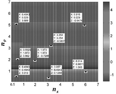
From Fig. 2 it follows that the value of the coupling coefficients depends on the value of $n_{x}$ and $n_{φ}$ . In this figure, it can been seen that the peak value of the coupling coefficients is related to the frequency ratio ( $n_{x}$ and $n_{φ}$ ) of the system, however, parameters $n_{x}$ and $n_{φ}$ are the function of the spring stiffness $k_{x}$ and $k_{ϕ}$ , respectively. In other words, the coupling coefficients are determined by the spring stiffness. Clearly, for $0.1 < n_{x} < 0.9$ and $0.1 < n_{φ} < 0.9$ , the vibration frequency of the system is less than the eigen-frequency of the system; in this case, the absolute value of $μ_{1},$ $μ_{2},$ $μ_{3}$ and $μ_{4}$ is smaller, which is denoted by before-resonance system. For $0.9 \leq n_{x} < 1.1$ and $0.9 \leq n_{φ} < 1.1$ , the vibration frequency of the system is approximately equal to the eigen-frequency of the system; in this case, the absolute value of $μ_{1}$ , $μ_{2}$ , $μ_{3}$ and $μ_{4}$ is far larger, which is denoted by resonance system. For $n_{x} \geq 1.1$ and $n_{φ} \geq 1.1$ , the vibration frequency of the system is larger than the eigen-frequency of the system; in this case, the value of $μ_{1}$ , $μ_{2}$ , $μ_{3}$ and $μ_{4}$ is also smaller, which is denoted by after-resonance system. Then, we can define the type of coupling of the system according to frequency ratio:

Type 1: system of before-resonance coupled before-resonance $(0.1 < n_{x} < 0.9$ and $0.1 < n_{φ} < 0.9$ );

Type 2: system of after-resonance coupled before-resonance $(0.1 < n_{x} < 0.9$ and $1.1 < n_{φ} < 7$ , or $1.1 < n_{x} < 7$ and $0.1 < n_{φ} < 0.9$ );

Type 3: system of after-resonance coupling after-resonance ( $1.1 < n_{φ} < 7$ and $1.1 < n_{x} < 7$ ).

Fig. 2The value of the coupling coefficients of the system for σ= 0.17, rm= 0.02 and β= 30°. In this figure, coordinate X represents the value of frequency ratio nx; coordinate Y represents the value of frequency ratio nφ; coordinate Z represents the value of coupling coefficients

The value of the coupling coefficients of the system for σ= 0.17, rm= 0.02 and β= 30°. In this figure, coordinate X represents the value of frequency ratio nx; coordinate Y represents the value of frequency ratio nφ; coordinate Z represents the value of coupling coefficients

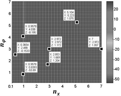
a) The value of $μ_{1}$ and $μ_{2}$

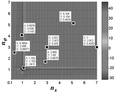
b) The value of $μ_{2}$

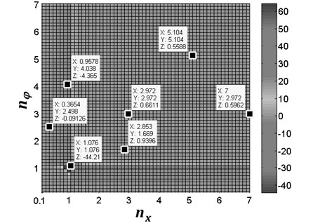
c) The value of $μ_{3}$

4. Synchronization and stability

In this section, we analyze the synchronization and stability of the system with theoretical method. As was already mentioned in Eq. (3), permits the family of synchronous solutions:

23

\{\begin{array}{l} φ_{1} = ω t + α_{1}, \\ φ_{2} = ω t + α_{2} . \end{array}

So Eq. (19) can be rewritten as:

24

\{\begin{array}{l} x = μ_{1} r_{m} r [c o s (ω t + α_{1}) - c o s (ω t + α_{2})] - μ_{2} σ r s i n (ω t + α_{2} - β), \\ φ_{3} = μ_{3} r_{m} r_{l} [c o s (ω t + α_{1}) - c o s (ω t + α_{2})] - μ_{4} σ r_{l} s i n (ω t + α_{2} - β) . \end{array}

Specifying parameter $α$ as the phase difference between the two rotors, we have:

25

α = α_{1} - α_{2} .

Consequently, the basic Eq. (4) is expressed as:

26

\{\begin{array}{l} \begin{array}{l} P_{1} = ⟨μ Φ_{1}⟩ = ⟨M_{e 1} - R_{e 1} - m_{1} r \ddot{x} s i n φ_{1}⟩ \\ = M_{e 1} - R_{e 1} - \frac{1}{2} m r^{2} ω^{2} [μ_{1} r_{m} s i n α + μ_{2} σ c o s (α + β)], \end{array} \\ P_{2} = ⟨μ Φ_{2}⟩ = ⟨M_{e 2} - R_{e 2} + m r [\ddot{x} s i n φ_{2} - l {\ddot{φ}}_{3} c o s (β - φ_{2}) + l {\dot{φ}}_{3}^{2} s i n (β - φ_{2})]⟩ \\ = M_{e 2} - R_{e 2} + \frac{1}{2} m_{2} r^{2} ω_{m}^{2} [μ_{1} r_{m} s i n α + μ_{2} σ c o s β + μ_{3} r_{m} c o s (α + β) - μ_{3} r_{m} c o s β] . \end{array}

During the synchronization state, consider the excessive torque $Z_{s} (ω)$ of the rotor to be zero:

27

Z_{s} (ω) = M_{e s} - R_{e s} = 0, (s = 1, 2) .

Therefore, according to Eqs. (25) and (26), further calculations lead to the following from:

28

\{\begin{array}{l} μ_{1} r_{m} s i n α + μ_{2} σ c o s (α + β) = 0, \\ μ_{1} r_{m} s i n α + μ_{3} r_{m} c o s (α + β) = (μ_{3} r_{m} - μ_{2} σ) c o s β . \end{array}

In terms of Eq. (22), we can obtain:

29

μ_{3} r_{m} = μ_{2} σ .

Thus the two formulas in Eq. (28) are identical. The synchronization occurs when the following equations are fulfilled:

30

μ_{1} s i n α + μ_{3} c o s (α + β) = 0 .

We can defined Eq. (30) as balance equation of synchronization of the system. Applying expansion of trigonometric function to Eq. (30), we have:

31

c o t α = \frac{μ_{3} s i n β - μ_{1}}{μ_{3} c o s β} .

If a solution of parameter $α$ exists in Eq. (31), the denominator of this equation should be nonzero. Therefore, there is a ‘critical point’, which can be expressed as:

32

β = k π + \frac{π}{2}, (k = 0, 1, 2, 3 \dots) .

When the installation angular of the pendulum rod is approximated or equal to this point, the absent-synchronization of the system will be appeared. Based on Eq. (31), the synchronization equation of the system, we can determine phase difference $α$ with numerical computations. Obviously, the value of the phase difference is related to the coupling coefficients ( $μ_{1}$ and $μ_{3}$ ) and the installation angle ( $β$ ). Moreover, parameters $μ_{1}$ and $μ_{3}$ are the function related to spring stiffness $k_{x}$ and $k_{φ}$ , which indicate that spring stiffness $k_{x}$ and $k_{φ}$ are the key parameters to determine phase difference $α$ .

Therefore, Eqs. (26) and (31) can be solved for synchronous velocity $ω_{m}$ of the motors and the phase difference between the two rotors, respectively. Then the phase difference between the two rotors can be obtained:

33

α = a r c c o t \frac{μ_{3} s i n β - μ_{1}}{μ_{3} c o s β} .

Now, let us consider the stability of the synchronous rotation for the rotors. With a subtraction for the two formulas in Eq. (26), one gets:

34

P_{1} - P_{2} = M_{e 1} - R_{e 1} - (M_{e 2} - R_{e 2}) - m r^{2} ω^{2} [μ_{1} r_{m} s i n α + μ_{3} r_{m} c o s (α + β)] .

Considering Eq. (34), the following criterion of synchronous stability is obtained from Eq. (6):

35

χ = \frac{\partial (P_{1} - P_{1})}{\partial α_{1}} = \frac{\partial (P_{1} - P_{1})}{\partial α} = - m r^{2} ω^{2} [μ_{1} r_{m} c o s α - μ_{3} r_{m} s i n (α + β)] < 0 .

Rearranging Eq. (35), the stability criterion of synchronization of the system can be simplified as:

36

μ_{1} c o s α - μ_{3} s i n (α + β) > 0 .

Only should the values of the system parameters satisfy the balance equation and the stability criterion of synchronization of the system, that the synchronous operation of the rotors can be implemented. In this case, the phase difference between the rotors is called as the stable phase difference.

5. Numerical discussions

The above-mentioned sections have given some theoretical discussions in the simplified form on synchronization problem for the vibration system that the two unbalanced rotors coupled with a pendulum rod. In this section, we will quantitatively analyze the results of the stable phase difference. The parameter values corresponding to general engineering application are as given in Tables 1, 2.

5.1. Theoretical solutions

The stiffness coefficients $k_{x}$ and $k_{φ}$ , which is separately converted to frequency ratio $n_{x}$ and $n_{φ}$ , have influence on the phase difference according to Eq. (30). Under the condition that the synchronization condition and stability criterion of two rotors (Eq. (30) and (36)) are satisfied, the stable phase difference can be determined by using numerical method.

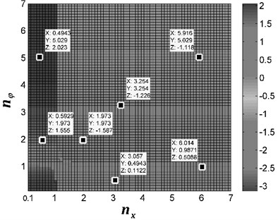
The influence of the frequency ratio on values of the stable phase difference is compared, considering the different values of the parameter $β$ , as shown in Fig. 3. According to Eqs. (22), (30) and (36), we have $μ_{2} = μ_{3} = 0$ when $β = 0$ , and the synchronization condition is simply expressed as $s i n α = 0$ , similarly, the synchronization stability criterion is rewritten as $μ_{1} c o s α > 0$ . Since $0.1 < n_{x} < 1$ and $μ_{1} < 0$ (in this case, $α = π$ ), it then follows that in before-resonance region ( $ω_{m} < ω_{x}$ ) the synphase motion is unstable and the antiphase motion is stable ([1] describes that the motion, as the existence of $α \in ($ – $π / 2, π / 2)$ , is call as synphase synchronization; and the motion, as the existence of $α \in (π / 2, 3 π / 2)$ , is call as antiphase synchronization). In after-resonance region ( $ω_{m} > ω_{x}$ ), on the contrary, (in this case, $α = 0$ ), the synphase synchronization is stable and the antiphase synchronization is unstable. As shown in Fig. 3(a), it is clear that the stable phase difference is equal to $π$ [rad] for $0.1 < n_{x} < 1$ (2.46×10⁶ $< k_{x} <$ 2.46×10⁸) and is equal to zero for $1 < n_{x} < 7$ ( $50307 < k_{x} <$ 2.46×10⁶). Note that parameter $n_{φ}$ has little influence on the value of stable phase difference; in other words, the phase difference is independent of the stiffness of the torque spring in the pendulum rod for $β =$ 0 [rad].

On the other hand, from Fig. 3(b), (c) and (d), it follows that the spring stiffness in the pendulum rod also determine the value of the phase difference when the value of parameter $β$ is nonzero. As shown in Fig. 3(b), considering $β = π / 6$ [rad], the antiphase synchronization exists when $0.1 < n_{x} < 1$ and $1 < n_{φ} < 7$ ; clearly, for $0.1 < n_{x} < 1$ and $0.1 < n_{φ} < 1$ , both antiphase and synphase synchronization appear; furthermore, in the interval $1 < n_{x} < 7$ and $0.1 < n_{φ} < 7$ , the two rotors always synchronize in synphase.

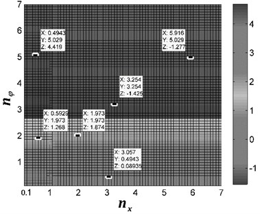
Fig. 3Stable phase difference with the theoretical computation. In this figure, coordinate X represents the value of frequency ratio nx; coordinate Y represents the value of frequency ratio nφ; coordinate Z represents the value of stable phase difference α

Stable phase difference with the theoretical computation. In this figure, coordinate X represents the value of frequency ratio nx; coordinate Y represents the value of frequency ratio nφ; coordinate Z represents the value of stable phase difference α

a) $β =$ 0 [rad]

b) $β = π / 6$ [rad]

c) $β = π / 3$ [rad]

d) $β = 5 π / 12$ [rad]

In the following calculations, the parameter values are the same as in the previous computations, except for $β$ , which is fixed to $β = π / 3$ [rad]. From Fig. 3(c) it follows that for this value of $β$ the rotors may synchronize either synphase or antiphase, also depending on the values of $n_{x}$ and $n_{φ}$ . The obtained results reveal that: in the interval $0.1 < n_{x} < 1$ and $0.1 < n_{φ} < 1$ , antiphase synchronization is implemented between the rotors; in the interval $0.1 < n_{x} < 1$ and $1 < n_{φ} < 7,$ both antiphase and synphase synchronization are remained; in the interval $1 < n_{x} < 7$ and for $1 < n_{φ} < 7$ , the two rotors will be synchronously operated in synphase state.

In the last computations, considering $β = 5 π / 12$ [rad] near the absent-synchronization point ( $β = π / 2$ [rad]), and the other parameter values are identical with the previous calculations. Fig. 3(d) depicts the value of the stable phase difference. In the figure, the value of the frequency ratio in the region of $0.1 < n_{x} < 1$ and $0.1 < n_{φ} < 1$ , antiphase rotation of the rotor is carried out; however, in the region of $1 < n_{x} < 7$ and $0.1 < n_{φ} < 2.7,$ both antiphase and synphase synchronization are appeared; finally, the frequency ratio in the other regions, synphase synchronization between the two rotors is locked.

5.2. Sample verifications

Further analyses have been performed by computer simulations to verify our theoretical solutions above, which can be carried out by applying the Runge-Kutaa routine with adaptive stepsize control to the dynamics Eq. (11). Here, the parameters of the two motors, supplied the power source at the same time, are assumed to be identical.

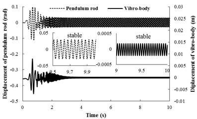
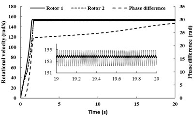
Fig. 4Simulation results for nx= 0.4943, nφ= 0.4943 and β=π/6

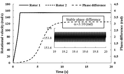
a) Rotational velocity and phase difference of the two rotors

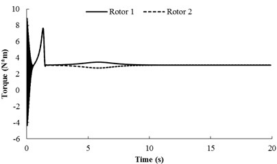
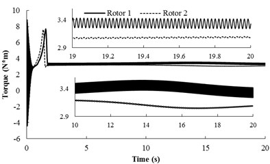
b) Torques of the two rotors

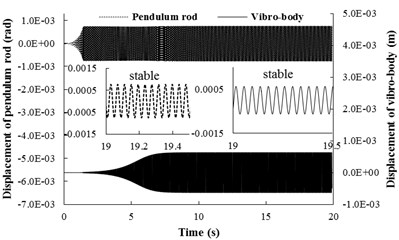
c) Displacement responds of the pendulum rod and the vibrating body

1) For $n_{x} =$ 0.4943, $n_{φ} =$ 0.4943 and $β = π / 6$ .

Simulation results for $n_{x} =$ 0.4943, $n_{φ} =$ 0.4943 and $β = π / 6$ are shown in Fig. 4, here, the spring stiffness is $k_{x} =$ 9859600 [N/m] and $k_{φ} =$ 976100 [N/rad]. The coupling type of the system belongs to type 1. When the two motor are supplied the electric source at the same time, the angular accelerations of the two rotors are equal each other (in Fig. 4(a)). The reason is that the inertia moments of the two rotors are identical and the spring stiffness is stronger. During the staring process of the system, the velocity difference exists between the two rotors, which leads to the phase difference unstable. However, when the angular velocities of the motors reach the operation value and the pendulum rod oscillate steadily, the synchronization phenomenon occurs. At this moment, the coupling torques (in Fig. 4(b)), making the phase difference $α$ stabilize at 3.10 [rad], are approximated to 3.08 [N⋅m]. In this case, the two motors rotate stably in antiphase synchronization, and the synchronous velocity is 153.8 [rad/s]. From Fig. 4(c) it follows the displacements of the pendulum rod and the vibrating body. It can be seen that the displacement responds of the pendulum rod and the vibrating body are stable, and the amplitudes of them are 7×10^-4 [rad] and 7×10^-4 [m], respectively. Comparing simulation results with Fig. 3(b), it should be noted that the value of the stable phase difference is in agreement with the results obtained for the case of theoretical solutions (i.e., the stable phase difference in Fig. 3(b) is equal to 3.013 [rad], here, the stable phase difference is equal to 3.10 [rad]).

2) For $n_{x} =$ 5.916, $n_{φ} =$ 5.029 and $β = π / 6$ .

This subsection refers to the case that the system of after-resonance is coupled with the after-resonance, for $n_{x} =$ 5.916, $n_{φ} =$ 5.029. In the simulation model, here the spring stiffness are $k_{x} =$ 65969 [N/m] and $k_{φ} =$ 1053 [N/rad], and the other parameter value is identical with Table 1. When the two motor are supplied the electric source at the same time, the angular accelerations of the two rotors are incompatible (in Fig. 5(a)) because of the larger amplitude of pendulum than that of condition 1. During the staring process of the system, the velocity difference obviously exists between the two rotors, which leads to unstable phase difference of the rotors. However, when the angular velocities of the motors reach the operation value and the pendulum rod oscillate steadily, the synchronization phenomenon occurs. At this moment, the coupling torques (in Fig. 5(b)), making the phase difference $α$ stabilize at –0.515 [rad], are approximated to 3.23 [N⋅m]. In this case, the two motors rotate stably in synphase synchronization, and the average synchronous velocity is 153.5 [rad/s]. It is noteworthy that the velocity fluctuation of rotor 2, installed in the pendulum, is stronger than rotor 2. This indicate that the larger amplitude of the pendulum results in the larger velocity fluctuation of the motor. From Fig. 5(c) it follows the displacements of the pendulum rod and the vibrating body. It is clear that when the rotation velocity of the two rotors pass through the resonant region of the coupling system, the resonant responses of the system in the $x$ - and $φ_{3}$ -direction are appeared in the starting process. In the synchronization state, the displacements of the pendulum rod and the vibrating body are stable, and the amplitudes of them are 0.02 [rad] and 2.5×10^-4 [m], respectively. Comparing simulation results with Fig. 3(b), the value of the stable phase difference by the computer simulations is according to the theoretical computations (i.e., the stable phase difference in Fig. 3(b) is equal to –0.5474 [rad], here, the stable phase difference is equal to –0.515 [rad]).

Fig. 5Simulation results for nx= 5.916, nφ= 5.029 and β=π/6

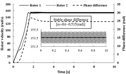
a) Rotational velocity and phase difference of the two rotors

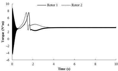
b) Torques of the two rotors

c) Displacement responds of the pendulum rod and the vibrating body

3) For $n_{x} =$ 5.916, $n_{φ} =$ 5.029 and $β = π / 2$ .

Importantly, the theoretical results in Eq. (32) have shown that around the ‘critical point’ $β = π / 2$ , the stable phase difference does not exist or is unstable. Moreover, the results can be supported by numerical simulations. We assume that $β = π / 2$ in the simulation model and the other parameter values is the same as condition 2. The numerical results are depicted in Fig. (6). During the staring process of the system, the velocity of rotor 1 is obviously larger than rotor 2 on account of the oscillation of the pendulum rod. When the angular velocities of the motors reach the operation value, however, coupling torques between the rotors is absent as $β = π / 2$ (as shown in Fig. 6(b), the torque of the two rotors is non-identical in all time-histories). Therefore, the phase difference between the rotors is unstable, as shown in Fig. 6(a). From Fig. 6(c), it follows the displacement responses of the pendulum rod and the vibrating body; it reveals that the unstable phase difference leads to the unstable displacement responses. Therefore, the system within such parameters unsuitably applied in the engineering.

Fig. 6Simulation results for nx= 5.916, nφ= 5.029 and β=π/2

a) Rotational velocity and phase difference of the two rotors

b) Torques of the two rotors

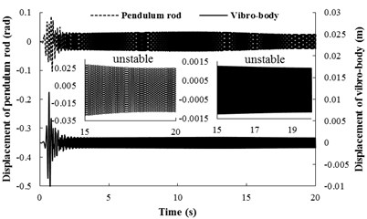
c) Displacement responds of the pendulum rod and the vibrating body

6. Conclusions

Based on our published literature, we have studied a model considering of two counter-rotating rotors coupled with a rigid pendulum rod and a vibrating body, which is horizontally connected to a fixed support by means of springs. In this paper, the dynamics equations of the system are converted into dimensionless equations, on which the synchronized state (i.e., synphase and antiphase synchronization of the rotors) have been investigated. Only should the values of the system parameters satisfy the synchronization balance equation and the stability criterion of synchronization of the system, the synchronization operation of the rotors can be implemented. Theoretical and numerical results have shown that the existence and stability of the synchronous state are influenced by the spring stiffness and the installation angular of the pendulum rod, which is verified by the computer simulations. Meanwhile, the existence of the ‘critical point’ ( $β = k π + π / 2$ , $(k =$ 0, 1, 2, 3… $)$ ) results in the absence of the coupling torques between the rotors. Therefore, the phase difference is unstable, which leads to the unstable displacement responses of the system.

The vibration system proposed in this paper may be applied to design new balanced elliptical vibrating screens, when their physics parameters satisfy the balance equation and the stability criterion of synchronization. In the early stage, for the developing and understanding the internal characteristics of the system, we only consider the vibrating body under the assumption of horizontal displacement. Will these results change if the vibrating body under multiple DOFs is taken into account? We believe that finding the answer to this question is the next step in challenging task of getting a complete understanding of synchronization in such system.

References

Blekhman I. I. Synchronization in Science and Technology. ASME Press, New York, 1988.

Search CrossRef
Arkady Pikovsky, Michael Rosenblum, Kurths J. Synchronization – A Universal Concept in Nonlinear Sciences. 2001.

Search CrossRef
Arenas A., Díaz-Guilera A., Kurths J., Moreno Y., Zhou C. Synchronization in complex networks. Physics Reports, Vol. 469, Issue 3, 2008, p. 93-153.

Search CrossRef
Zhang H., Wang X. Y., Lin X. H., Liu C. X. Stability and synchronization for discrete-time complex-valued neural networks with time-varying delays. Plos One, Vol. 9, Issue 4, 2014, p. 6.

Search CrossRef
Yuan W.-J., Zhou C. Interplay between structure and dynamics in adaptive complex networks: emergence and amplification of modularity by adaptive dynamics. Physical Review E, Vol. 84, Issue 1, 2011.

Search CrossRef
Peña Ramirez J., Aihara K., Fey R. H. B., Nijmeijer H. Further understanding of Huygens coupled clocks: the effect of stiffness. Physica D: Nonlinear Phenomena, Vol. 270, 2014, p. 11-19.

Search CrossRef
Jovanovic V., Koshkin S. Synchronization of Huygens clocks and the Poincaré method. Journal of Sound and Vibration, Vol. 331, Issue 12, 2012, p. 2887-2900.

Search CrossRef
Koluda P., Perlikowski P., Czolczynski K., Kapitaniak T. Synchronization configurations of two coupled double pendula. Communications in Nonlinear Science and Numerical Simulation, Vol. 19, Issue 4, 2014, p. 977-990.

Search CrossRef
Dilão R. Anti-phase synchronization and ergodicity in arrays of oscillators coupled by an elastic force. The European Physical Journal Special Topics, Vol. 223, Issue 4, 2014, p. 665-676.

Search CrossRef
Marcheggiani L., Chacón R., Lenci S. On the synchronization of chains of nonlinear pendula connected by linear springs. The European Physical Journal Special Topics, Vol. 223, Issue 4, 2014, p. 729-756.

Search CrossRef
Wen J. F. B. C., Zhao C. Y. Synchronization and Controlled Synchronization in Engineering. Science Press, Beijing, 2009.

Search CrossRef
Zhang X., Wen B., Zhao C. Synchronization of three non-identical coupled exciters with the same rotating directions in a far-resonant vibrating system. Journal of Sound and Vibration, Vol. 332, Issue 9, 2013, p. 2300-2317.

Search CrossRef
Zhang X., Wen B., Zhao C. Vibratory synchronization and coupling dynamic characteristics of multiple unbalanced rotors on a mass-spring rigid base. International Journal of Non-Linear Mechanics, Vol. 60, 2014, p. 1-8.

Search CrossRef
Sperling L., Ryzhik B., Linz C., Duckstein H. Simulation of two-plane automatic balancing of a rigid rotor. 2nd International Conference on Control of Oscillations and Chaos (COC-2000), Vol. 58, 2002, p. 351-365.

Search CrossRef
Balthazar J. M., Felix J. L. P., Brasil R. M. L. R. F. Short comments on self-synchronization of two non-ideal sources supported by a flexible portal frame structure. Journal of Vibration and Control, Vol. 10, Issue 12, 2004, p. 1739-1748.

Search CrossRef
Balthazar J. M., Felix J. L. P., Brasil R. M. Some comments on the numerical simulation of self-synchronization of four non-ideal exciters. Applied Mathematics and Computation, Vol. 164, Issue 2, 2005, p. 615-625.

Search CrossRef
Djanan A. A. N., Nbendjo B. R. N., Woafo P. Effect of self-synchronization of DC motors on the amplitude of vibration of a rectangular plate. The European Physical Journal Special Topics, Vol. 223, Issue 4, 2014, p. 813-825.

Search CrossRef

About this article

Received

21 March 2015

Accepted

15 July 2015

Published

15 August 2015

SUBJECTS

Chaos, nonlinear dynamics and applications

Keywords

synchronization

stability

rotors

pendulum rod

Acknowledgements

This study is supported by National Natural Science Foundation of China (Grant No. 51074132).

This is an open access article distributed under the Creative Commons Attribution License, which permits unrestricted use, distribution, and reproduction in any medium, provided the original work is properly cited.