On the natural frequency and vibration mode of composite beam with non-uniform cross-section

Li, Botong; Dong, Longlei; Zhu, Liangliang; Chen, Xi

Journal of Vibroengineering

Browse Journal

Submit article

Published: 15 August 2015

Check for updates

On the natural frequency and vibration mode of composite beam with non-uniform cross-section

Botong Li¹

Longlei Dong²

Liangliang Zhu³

Xi Chen⁴

¹College of Mechanical Engineering, Beijing University of Technology, Beijing 100124, China

²State Key Laboratory for Strength and Vibration of Mechanical Structures, School of Aerospace, Xi’an Jiaotong University, Xi’an 710049, China

^{3, 4, 1}International Center for Applied Mechanics, SV Lab, School of Aerospace, Xi’an Jiaotong University, Xi’an 710049, China

⁴Department of Earth and Environmental Engineering, Columbia University, New York, NY 10027, USA

Corresponding Author:

Xi Chen

Cite the article Download PDF

Downloads 1514

Abstract

In this paper, the vibratory properties and expression of natural modes of laminated composite beam with variable cross-section ratios of elastic modulus and density along the axis of the beam have been investigated via theoretical analysis. Based on the generalized Hamilton principle, the longitudinal and transverse vibration equations have been deduced by the means of variational method. Then, the natural frequencies of longitudinal and transverse vibration modes have been obtained using the method of power series, which agree well with finite element simulations. The first-order natural frequencies of longitudinal and transverse of composite beams are plotted as a function of the elastic modulus or densities difference of two components. With distinct material characteristics, the effect of shape factor on the first and second order lateral modes of composite beam is also revealed. In addition, the study shows that the boundary conditions impose a strong effect on the shape factor. The method presented in this paper is not only suitable for the laminated composite beam with variable cross-section, but will also be applicable to more general cases of composite beams of complex geometry and component in vibration mechanics. This controllable vibration performance achieved in this paper may shed some light on and stimulate new architectural design of composite engineering structures.

1. Introduction

In mechanical, aerospace and civil structures and vehicles, laminated structural components have received wide applications thanks to their distinct advantages of high strength, stiffness-to-weight ratios and high bending rigidity [1, 2]. An important example is the widely used steel-concrete components in bridges [3, 4]. For structural applications, the eigenmodes and vibration characteristics of composite beams are of great importance [5]. Extensive theoretical and numerical approaches were carried out to explore the natural frequencies of laminated structures. Tseng et al. [6] applied the stiffness analysis method involving shear deformation and rotation inertia to determine the natural frequencies of laminated beams with arbitrary curvatures. Banerjee [7] presented the frequency equation and mode shapes of composite Timoshenko beams by symbolic computing. Rao et al. [8] proposed a higher-order mixed theory for determining natural frequencies of several laminated simply supported beams. Chen et al. [9] combined the state space method and the differential quadrature method for freely vibrating laminated beams. An excellent overview of recent advances in straight and curved composite beam models may be found in [10]. Wu and Chen [11] and Qu et al. [12] compared a few free vibration modes of laminated beams using the shear deformation-based theories. By using the Rayleigh-Ritz (R-R) method, Gunda et al. [13] studied large amplitude vibration of laminated composite beam with symmetric and asymmetric layup orientations.

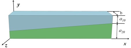
Most previous studies focused on composite beams with uniform axial properties, while composite beams with variable cross-sections may be needed to better fit the stress distribution or to achieve a better structural performance [14-17]. Present study emphasizes the normal mode analysis of composite beam with non-uniform constituent cross-section properties. The attention is limited to composite beams with a constant overall geometrical section dimension, but the height ratio between the components varies along the axial direction (Fig. 1), the configuration of which is similar to the widely used and studied scarf joint technique for fabricating composite structures [18-20]. It is noted that the algorithms presented here are also applicable to study other composite beams with more complex cross-section properties, for example, the jagged joint interface between two components.

Any general structural deformation can be regarded as a superposition of its fundamental normal modes, therefore, the present study emphasizes the normal mode analysis of composite beam with non-uniform constituent cross-section properties. To focus on the effect of constituent ratio, the attention is limited to composite beams with a constant overall geometrical section dimension, but the height ratio between the components varies along the axial direction (Fig. 1).

Many previous analytical and computational studies focused on the nonlinear vibration equations, using differential quadrature method (DQM) [21-22], dynamic stiffness method [23], finite element method (FEM) [24] and finite difference method [25], etc. In this paper, we adopt the variational method to obtain the kinetic equations of composite beams with variable cross-section ratios of elastic modulus, and to deduce the analytical expression of natural modes of longitudinal and transverse vibrations. Numerical validations are carried out using finite element simulations.

Though this study focuses on a rather simple composite beam with two components attached on their inclined surface (Fig. 1), the algorithms presented here can be easily extended to be applicable to studying composite beams of complex geometry and multiple components. One example is to study the vibration mode and frequency of the helicopter rotor blades which consist of multiple different material components and each component’s cross-section may be varying along its length direction. This study is also intended to stimulate new design of composite structures. A widely used composite beam structure is the composite bridges usually composed of a uniform layer of steel, a uniform layer of concrete and probably a uniform layer of fiber reinforced polymer deck. We believe that a more appropriate design of the bridge with varying cross-section of each material component (for example, increasing the thickness of the concrete layer in the middle region of the bridge) may be able to spread the load on the bridge, thus exploiting the inherent advantages of each of its material. Besides, it would be routine to analyze the natural frequency and vibration mode of a number of composite structures with various joint interface geometries [14, 17] based on the formulas presented here.

2. Modeling and mathematics formulation

Consider a beam of rectangular cross section, composed of two materials with their ratio changing along the axial direction. This is equivalent to bonding two rectangular beams with variable cross section, (Fig. 1). Such a configuration may be applicable to the composite components in bridges to allow a better fitting of the bending moment distribution of the bridge due to external loading or used as a scarf joint for composite structures. It is worth noting that our normal mode analysis algorithms presented below are not limited to this configuration, but can be easily adapted to study other composite beams with more complex $x$ - $y$ cross-section properties. All beams considered here are Bernoulli-Euler beams.

The elastic modulus, cross-sectional area, moment of inertia, length and density of the upper beam are $E_{1}$ , $A_{1} (x)$ , $I_{1} (x)$ , $l$ , $ρ_{1}$ , respectively, while the ones of lower beam are $E_{2}$ , $A_{2} (x)$ , $I_{2} (x)$ , $l$ , $ρ_{2}$ . The width of the beam is $b$ . Thus, the cross-sectional areas of upper and lower beams are:

1

A_{1} (x) = (a_{10} + k x) b,

A_{2} (x) = (a_{20} - k x) b,

while $a_{10} + a_{20} = a$ and $k = (a_{20} - a_{10}) / l$ .

The moment of inertia of beams can be derived as:

2

I_{1} (x) = \frac{b {(a_{10} + k x - \frac{a}{2})}^{3}}{3} + \frac{b a^{3}}{24}, I_{2} (x) = \frac{b a^{3}}{24} - \frac{b {(\frac{a}{2} - a_{20} + k x)}^{3}}{3} .

According to the neutral plane assumption, the longitudinal (axial) deformation $u$ of upper beam and lower beam are the same. We can also obtain the similar conclusion with the transverse deformation $w$ . Shear deformation is neglected.

The kinetic energy of the system is:

3

T_{1} = \frac{[\int_{0}^{1} ρ_{1} A_{1} (x) ({\dot{u}}_{1}^{2} + {\dot{w}}_{1}^{2}) d x]}{2}, T_{2} = \frac{[\int_{0}^{1} ρ_{2} A_{2} (x) ({\dot{u}}_{2}^{2} + {\dot{w}}_{2}^{2}) d x]}{2} .

The energy of the system is:

4

V_{1} = \frac{\{\int_{0}^{1} [E_{1} A_{1} (x) {(\frac{\partial u_{1}}{\partial x})}^{2} + E_{1} I_{1} (x) {(\frac{\partial^{2} w_{1}}{\partial x^{2}})}^{2}] d x\}}{2},

5

V_{2} = \frac{\{\int_{0}^{1} [E_{2} A_{2} (x) {(\frac{\partial u_{2}}{\partial x})}^{2} + E_{2} I_{2} (x) {(\frac{\partial^{2} w_{2}}{\partial x^{2}})}^{2}] d x\}}{2} .

Using variational principle, one obtains:

6

δ \int_{t_{0}}^{t_{1}} T d t = δ \int_{t_{0}}^{t_{1}} (T_{1} + T_{2}) d t = δ \int_{t_{0}}^{t_{1}} \frac{[\int_{0}^{1} [ρ_{1} A_{1} (x) + ρ_{2} A_{2} (x)] ({\dot{u}}_{}^{2} + {\dot{w}}_{}^{2}) d x]}{2} d t

= \int_{t_{0}}^{t_{1}} \int_{0}^{1} [ρ_{1} A_{1} (x) + ρ_{2} A_{2} (x)] (- \ddot{u} δ u - \ddot{w} δ w) d x d t,

7

δ \int_{t_{0}}^{t_{1}} V d t = δ \int_{t_{0}}^{t_{1}} (V_{1} + V_{2}) d t = δ \int_{t_{0}}^{t_{1}} \frac{1}{2} \int_{0}^{1} [E_{1} A_{1} (x) + E_{2} A_{2} (x)] {(\frac{\partial u}{\partial x})}^{2} d x d t

+ δ \int_{t_{0}}^{t_{1}} \frac{1}{2} \int_{0}^{1} [E_{1} I_{1} (x) + E_{2} I_{2} (x)] {(\frac{\partial^{2} w}{\partial x^{2}})}^{2} d x d t

= - \int_{t_{0}}^{t_{1}} \int_{0}^{1} \frac{\partial}{\partial x} \{[E_{1} A_{1} (x) + E_{2} A_{2} (x)] \frac{\partial u}{\partial x}\} δ u d x d t

+ \int_{t_{0}}^{t_{1}} \int_{0}^{1} [E_{1} I_{1} (x) + E_{2} I_{2} (x)] (\frac{\partial^{2} w}{\partial x^{2}}) δ (\frac{\partial^{2} w}{\partial x^{2}}) d x d t

= \int_{t_{0}}^{t_{1}} \{\int_{0}^{1} - \frac{\partial}{\partial x} \{[E_{1} A_{1} (x) + E_{2} A_{2} (x)] \frac{\partial u}{\partial x}\} δ u d x

+ \int_{0}^{1} \frac{\partial^{2}}{\partial x^{2}} \{[E_{1} I_{1} (x) + E_{2} I_{2} (x)] (\frac{\partial^{2} w}{\partial x^{2}})\} δ w d x\} d t .

Based on the generalized Hamilton principle, the following equations with independent $δ u$ and $δ w$ are obtained:

8

[ρ_{1} A_{1} (x) + ρ_{2} A_{2} (x)] \frac{\partial^{2} u}{\partial t^{2}} - [E_{1} \frac{\partial A_{1} (x)}{\partial x} + E_{2} \frac{\partial A_{2} (x)}{\partial x}] \frac{\partial u}{\partial x}

- [E_{1} A_{1} (x) + E_{2} A_{2} (x)] \frac{\partial^{2} u}{\partial x^{2}} = 0,

9

[ρ_{1} A_{1} (x) + ρ_{2} A_{2} (x)] \frac{\partial^{2} w}{\partial t^{2}} + [E_{1} I_{1} (x) + E_{2} I_{2} (x)] \frac{\partial^{4} w}{\partial x^{4}}

+ 2 [E_{1} \frac{\partial I_{1} (x)}{\partial x} + E_{2} \frac{\partial I_{2} (x)}{\partial x}] \frac{\partial^{3} w}{\partial x^{3}} + [E_{1} \frac{\partial^{2} I_{1} (x)}{\partial x^{2}} + E_{2} \frac{\partial^{2} I_{2} (x)}{\partial x^{2}}] \frac{\partial^{2} w}{\partial x^{2}} = 0 .

Fig. 1Beams with different cross-sectional areas

3. Mathematical transformation and calculation

3.1. The longitudinal deformation equation

The longitudinal deformation equation is considered first. From Eq. (8), it is assumed that the main vibration mode of beam is:

10

u (x, t) = U (x) b s i n (ω t + φ) .

Combining Eqs. (8) and (10):

11

U'' + \frac{α_{2} U^{'}}{(α_{1} + α_{2} x)} + \frac{(α_{3} + α_{4} x) ω^{2} U}{(α_{1} + α_{2} x)} = 0,

where $α_{1} = (E_{1} a_{10} + E_{2} a_{20}) b$ , $α_{2} = (E_{1} - E_{2}) k b$ , $α_{3} = (ρ_{1} a_{10} + ρ_{2} a_{20}) b$ , $α_{4} = (ρ_{1} - ρ_{2}) k b$ . Obviously, $α_{2} \neq 0$ . Assume that:

12

E_{1} > E_{2} .

It follows that $α_{2} > 0$ .

In Eq. (11), $α_{2} / (α_{1} + α_{2} x)$ and $(α_{3} + α_{4} x) ω^{2} / (α_{1} + α_{2} x)$ are analytical as $x \in [0, l],$ which may be solved using power series. Suppose that:

13

U = \sum_{n = 0}^{\infty} a_{n} x^{n} .

Substitute Eq. (13) into Eq. (11):

14

\sum_{n = 2}^{\infty} α_{1} n (n - 1) a_{n} x^{n - 2} + \sum_{n = 2}^{\infty} α_{2} n (n - 1) a_{n} x^{n - 1} + \sum_{n = 1}^{\infty} α_{2} n a_{n} x^{n - 1}

+ \sum_{n = 0}^{\infty} α_{3} ω^{2} a_{n} x^{n} + \sum_{n = 0}^{\infty} α_{4} ω^{2} a_{n} x^{n + 1} = 0 .

To obtain the solution, make each power coefficient of $x$ equal to zero, leads to:

15

a_{2} = \frac{- α_{3} ω^{2} a_{0} - α_{2} a_{1}}{2 α_{1}}, \dots, a_{r + 2} = \frac{- α_{2} (r + 1)^{2} a_{r + 1} - α_{3} ω^{2} a_{r} - α_{4} ω^{2} a_{r - 1}}{α_{1} (r + 2) (r + 1)}, r \geq 1 .

$a_{0}$ and $a_{1}$ are different constants.

Assuming that the beam is stationary initially:

16

u (x, 0) = 0 .

Substitute Eq. (16) into Eq. (10), one deduces $φ = 0$ .

Suppose the one end of the beam is fixed while the other is free. This kind of boundary condition is taken as an example in the calculating process:

17

U (0) = 0, U' (l) = 0 .

The fundamental modes of the system are:

18

U_{i} (x) = \sum_{n = 1}^{\infty} a_{n} (ω_{i}) x^{n}, i = 1, 2, \dots .

The frequency equation is:

19

\sum_{n = 1}^{\infty} n a_{n} (ω) l^{n - 1} = 0 .

Thus:

20

u (x, t) = \sum_{i = 1}^{\infty} U_{i} (x) b_{i} s i n (ω_{i} t) .

3.2. The transverse deformation equation

The transverse deformation is explored next. The main vibration equation is:

21

w (x, t) = Y (x) b s i n (ω t + φ) .

Substitute it into Eq. (9):

22

(β_{1} x^{3} + β_{2} x^{2} + β_{3} x + β_{4}) Y^{I V} + (6 β_{1} x^{2} + 4 β_{2} x + 2 β_{3}) Y'''

+ (6 β_{1} x + 2 β_{2}) Y'' - (α_{3} + α_{4} x) ω^{2} Y = 0,

where:

23

α_{3} = (ρ_{1} a_{10} + ρ_{2} a_{20}) b, α_{4} = (ρ_{1} - ρ_{2}) k b,

β_{1} = (E_{1} - E_{2}) \frac{b k^{3}}{3}, β_{2} = b k^{2} [E_{1} (a_{10} - \frac{a}{2}) - E_{2} (\frac{a}{2} - a_{20})],

β_{3} = b k [E_{1} {(a_{10} - \frac{a}{2})}^{2} - E_{2} {(\frac{a}{2} - a_{20})}^{2}],

β_{4} = b \{[E_{1} {(a_{10} - \frac{a}{2})}^{3} - E_{2} {(\frac{a}{2} - a_{20})}^{3}] + \frac{(E_{1} + E_{2}) a^{3}}{8}\} / 3 .

Suppose Eq. (22) has the solution in the form of (see Appendix for justification):

24

Y = \sum_{n = 0}^{\infty} a_{n} x^{n}, 0 \leq x \leq l .

Substitute the above equation into Eq. (22), yields:

25

\sum_{n = 4}^{\infty} β_{1} n (n - 1) (n - 2) (n - 3) a_{n} x^{n - 1} + \sum_{n = 4}^{\infty} β_{2} n (n - 1) (n - 2) (n - 3) a_{n} x^{n - 2}

+ \sum_{n = 4}^{\infty} β_{3} n (n - 1) (n - 2) (n - 3) a_{n} x^{n - 3} + \sum_{n = 4}^{\infty} β_{4} n (n - 1) (n - 2) (n - 3) a_{n} x^{n - 4}

+ \sum_{n = 3}^{\infty} 6 β_{1} n (n - 1) (n - 2) a_{n} x^{n - 1} + \sum_{n = 3}^{\infty} 4 β_{2} n (n - 1) (n - 2) a_{n} x^{n - 2}

+ \sum_{n = 3}^{\infty} 2 β_{3} n (n - 1) (n - 2) a_{n} x^{n - 3} + \sum_{n = 2}^{\infty} 6 β_{1} n (n - 1) a_{n} x^{n - 1}

+ \sum_{n = 2}^{\infty} 2 β_{2} n (n - 1) a_{n} x^{n - 2} - \sum_{n = 0}^{\infty} α_{3} ω^{2} a_{n} x^{n} - \sum_{n = 0}^{\infty} α_{4} ω^{2} a_{n} x^{n + 1} = 0 .

To obtain the solution, set each power coefficient of $x$ equal to zero, thus:

26

a_{4} = \frac{(α_{3} ω^{2} a_{0} - 4 β_{2} a_{2} - 12 β_{3} a_{3})}{24 β_{4}},

\dots,

a_{r + 4} = \frac{I_{r + 4}}{β_{4} (r + 4) (r + 3) (r + 2) (r + 1)},

I_{r + 4} = - β_{3} (r + 3) (r + 2)^{2} (r + 1) a_{r + 3} - β_{2} (r + 2)^{2} (r + 1)^{2} a_{r + 2}

- β_{1} (r + 2) (r + 1)^{2} r a_{r + 1} + α_{3} ω^{2} a_{r} + α_{4} ω^{2} a_{r - 1},

r \geq 1 .

$a_{0}$ , $a_{1}$ , $a_{2}$ and $a_{3}$ are different constant. Some boundary conditions are listed in order to discuss the problem further.

Assuming that the beam is stationary initially:

27

w (x, 0) = 0 .

Substitute Eq. (27) into Eq. (21), yields $φ = 0$ . Suppose the one end of the beam is fixed while the other is free:

28

Y (0) = 0, Y^{'} (0) = 0, Y^{''} (l) = 0, Y''' (l) = 0 .

The main modes for the systems are obtained:

29

Y_{i} (x) = \sum_{n = 2}^{\infty} a_{n} (ω_{i}) x^{n}, i = 1, 2, \dots .

The frequency equation is:

30

\sum_{n = 2}^{\infty} n (n - 1) a_{n} (ω) l^{n - 2} = \sum_{n = 3}^{\infty} n (n - 1) (n - 2) a_{n} (ω) l^{n - 3} = 0 .

Thus:

31

w (x, t) = \sum_{i = 1}^{\infty} Y_{i} (x) b_{i} \sin (ω_{i} t) .

4. Results and discussion

To compare with the results obtained by methods mentioned above, finite element simulations using ABAQUS [26] are employed to calculate both the first-order longitudinal and transverse natural modes of beams in six cases. Data in Table 1 reveals the relative difference between the analytical results and the finite element results. In the analytical procedure, a seventh-order polynomial is adopted in the equations.

Table 1Comparison between ABAQUS results and ones obtained by analytical methods

$a_{10} = a_{20} =$ 0.05 m	Longitudinal frequency			Transverse frequency
$a_{10} = a_{20} =$ 0.05 m	Analysis (rad/s)	Abaqus (rad/s)	Difference	Analysis (rad/s)	Abaqus (rad/s)	Difference
$ρ_{1} = ρ_{2} =$ 7.8×10³ kg/m³ $E_{1} = E_{2} =$ 200×10⁹ Pa	8063.5	7953.7	1.36 %	512.7	509.7	0.59 %
$ρ_{1} = ρ_{2} =$ 7.8×10³kg/m³ $E_{1} =$ 200×10⁹ Pa $E_{2} =$ 150×10⁹ Pa	7542.7	7439.7	1.37 %	480.3	473.0	1.52 %
$ρ_{1} = ρ_{2} =$ 7.8×10³kg/m³ $E_{1} =$ 200×10⁹ Pa $E_{2} =$ 100×10⁹ Pa	6983.2	6886.2	1.39 %	436.0	422.4	3.12 %
$ρ_{1} = ρ_{2} =$ 8.0×10³kg/m³ $E_{1} = E_{2} =$ 200×10⁹ Pa	7962.3	7853.7	1.36 %	506.2	503.2	0.59 %
$ρ_{1} =$ 8.0×10³kg/m³ $ρ_{2} =$ 6.0×10³kg/m³ $E_{1} = E_{2} =$ 200×10⁹ Pa	8512.0	8395.5	1.36 %	541.2	540.0	0.22 %
$ρ_{1} =$ 8.0×10³kg/m³ $ρ_{2} =$ 4.0×10³kg/m³ $E_{1} = E_{2} =$ 200×10⁹ Pa	9194.0	9066.4	1.38 %	584.6	581.0	0.62 %

4.1. The longitudinal frequency

Table 2 reveals the effect of shape factor $a_{10} / a_{20}$ on the frequency, as it can be seen from the charts, the boundary conditions imposes a strong effect on the shape factor. If both beam ends are fixed (or free), the longitudinal frequencies of the composite beam have little difference when the shape factors $a_{10} / a_{20}$ are reciprocal. Only with mixed boundary conditions, can frequencies vary according to the shape factor $a_{10} / a_{20}$ . In addition, with the same material characteristics and shape size, the boundary conditions of both ends fixed and free share no differences.

In Fig. 2(a), the first-order natural frequency of composite beams is examined. The elastic modulus of the upper beam is fixed at $E_{1} =$ 200×10⁹ Pa, while the elastic modulus of the lower beam is decreased (that is, $E_{1} - E_{2}$ rises from 0 to 100 (×10⁹ Pa)), which leads to the declination of the first-order natural frequency of composite beams. For comparison, if a reference beam is made by a uniform material whose elastic modulus is the average of the upper and the lower beam, a set of the first-order natural frequency of the uniform beam can be obtained (see the blue curve of reference results in Fig. 2(a)). From Fig. 2(a), the first-order natural frequency of the composite beam is considerably different than that of the reference uniform beam, that is, the difference between blue and black curve is especially significant. The black one composited of two bonded uniform beams, while the blue one is a uniform beam whose elastic modulus is the average of the two prior components. This difference implies nonlinear coupling between the longitudinal modes of the two component beams. The shape gradient also plays an important role in the natural frequency. In this case when the boundary condition is selected as fixed in the left and free in the right, the frequency is higher as $a_{10} / a_{20}$ rises.

Table 2Effects of the shape factor on the longitudinal frequency with different boundary conditions

		Fixed in both left and right	Free in both left and right	Fixed in left and free in right
$ρ_{1} = ρ_{2} =$ 7.8×10³kg/m³ $E_{1} =$ 200×10⁹ Pa $E_{2} =$ 100×10⁹ Pa	$a_{10} / a_{20} = 1 / 3$	13710.0	13725.0	6630.6
	$a_{10} / a_{20} = 1 / 1$	13761.0	13758.0	6886.2
	$a_{10} / a_{20} = 3 / 1$	13710.0	13725.0	7096.8
$ρ_{1} =$ 8.0×10³kg/m³ $ρ_{2} =$ 4.0×10³kg/m³ $E_{1} = E_{2} =$ 200×10⁹ Pa	$a_{10} / a_{20} = 1 / 3$	18187.0	18187.0	8873.6
	$a_{10} / a_{20} = 1 / 1$	18119.0	18115.0	9066.4
	$a_{10} / a_{20} = 3 / 1$	18111.0	18188.0	9386.3

In Fig. 2(b), the first-order natural frequency of composite beam is plotted as a function of the densities difference of two components. As expected, the first-order natural frequency of composite beams rises with the reduction of density of lower beam. The blue curve of reference solution in Fig. 2(b) is that of a uniform beam whose density is the average between upper and lower beam. Obviously the reference results have a significant difference not only from the composite beam with constant cross-section but also from varying cross-section composite beam. And the first-order natural frequency is greater when the size gradient gets bigger.

Fig. 2The first-order longitudinal frequency of beams with different cross-sectional areas; a10+a20=a= 0.1 m, l= 1 m

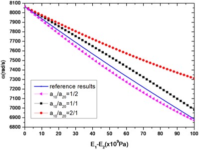
a) $E_{1} =$ 200×10⁹ Pa, $ρ_{1} = ρ_{2} =$ 7.8×10³ kg/m³

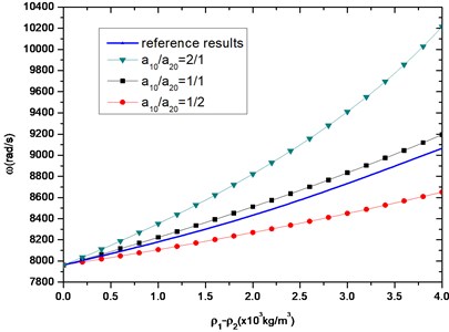
b) $E_{1} = E_{2} =$ 200×10⁹ Pa, $ρ_{1} =$ 8.0×10³ kg/m³

4.2. The transverse frequency and mode of vibration

Table 3 reveals the effects of the shape factor on transverse frequency with four representative boundary conditions combined by fixed, simple supported, and free conditions.

If the composite beam conditions at both ends are the same, the transverse frequency is the same when the shape factors $a_{10} / a_{20}$ are reciprocal, owing to the mirror symmetry. When the left end is fixed, and the right end sets free, the transverse frequency of composite beam varies obviously according to the shape factor $a_{10} / a_{20}$ . Therefore, the impacts of physical characteristic and shape properties on the transverse frequency with the left-fixed and right-free boundary conditions are discussed on the following section.

Fig. 3 shows the effect of physical properties and constituent ratio on the transverse frequency of the composite beam. For a composite beam with left end fixed and right end free, if one wants to improve the transverse frequency, a lower beam with bigger modulus or smaller density can be selected without changing the upper beam. Alternatively, one can tune the transverse frequency by changing the shape factor (constituent ratio along the axial direction) of the composite beam. The bigger the shape factor $a_{10} / a_{20}$ is, the greater the transverse frequencies of the composite beam are.

Table 3Effects of the shape factor on the transverse frequency with different boundary conditions

		Left and right fixed	Left (fixed) right (simple-supported)	Left and right freely supported	Left (fixed) right (free)
$ρ_{1} = ρ_{2} =$ 7.8×10³kg/m³ $E_{1} =$ 200×10⁹ Pa $E_{2} =$ 100×10⁹ Pa	$a_{10} / a_{20} = 1 / 3$	2582.9	1995.6	1646.5	419.8
	$a_{10} / a_{20} = 1 / 1$	3521.3	2679.8	2191.4	551.0
	$a_{10} / a_{20} = 3 / 1$	2566.4	2010.9	1650.3	421.1
$ρ_{1} =$ 8.0×10³kg/m³ $ρ_{2} =$ 4.0×10³kg/m³ $E_{1} = E_{2} =$ 200×10⁹ Pa	$a_{10} / a_{20} = 1 / 3$	3527.6	2713.5	2195.0	579.3
	$a_{10} / a_{20} = 1 / 1$	2582.9	2050.0	1646.5	428.6
	$a_{10} / a_{20} = 3 / 1$	3521.3	2740.6	2191.4	610.1

Fig. 3The first-order transverse frequency with a10+a20=a= 0.1 m, l= 1 m

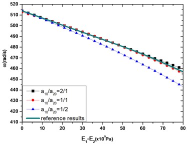
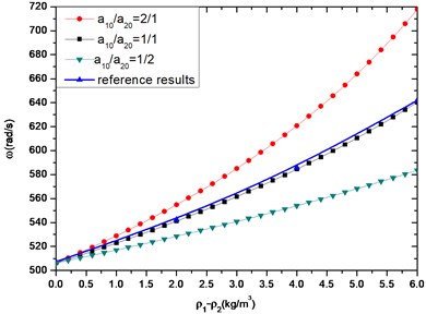
Fig. 4The mode of vibration of beams with different cross-sectional areas; E1= 200×109 Pa, E2= 1×109 Pa, ρ1=ρ2= 7.8×103 kg/m3, a10+a20=a= 0.1 m, l= 1 m

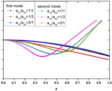
Comparing with a reference beam whose physical characteristics are the average of the ones of upper and lower beams, when changing the modulus of composite beam, the reference solutions of the single beam can be observed in Fig. 3. As the modulus of the lower beam varies, the reference results are close to the transverse frequency of composite beam with a shape factor of $a_{10} / a_{20} = 1 / 1$ , while as the density of the lower beam varies, the reference solution is close to the frequency of the composite beam with a shape factor of $a_{10} / a_{20} = 1 / 1$ . Fig. 4 reveals the effect of shape factor on the first and second order lateral modes of composite beam with distinct material characteristics. The left boundary condition is fixed, while the right is free. In this case, the modulus of upper beam is taken as $E_{1} =$ 200×10⁹ Pa, while the lower is $E_{2} =$ 1×10⁹ Pa, mimicking metal-polymer composite. For the first mode, the shape factor $a_{10} / a_{20}$ effect is small; however, for the second mode, the decrease of shape factor $a_{10} / a_{20}$ can induce the composite beam to bend more severely. At this time, the deformation of the composite beam becomes more exaggerated with a larger curvature.

Authors Botong Li and Longlei Dong made equal contribution.

5. Conclusions

Using the variational method the kinetic equations of composite beams are obtained, and analytical expressions on natural frequencies of longitudinal and transverse vibration of composite beams are deduced by using the method of power series. Finite element simulation is used to verify the theoretical framework. Effects of gradient ratio between components along the axial direction on the natural frequencies of composite beams are revealed, and the first and second order transverse modes of composite beams are drawn. Some of the important findings of the paper are:

1) When the elastic modulus of lower beam is decreased, both the longitudinal and transverse first-order natural frequencies of composite beams tend to decline, while they rise with the reducing of density of lower beam.

2) The shape gradient plays an important role in the natural frequency. For example, in a case where the left end is fixed and the right end is free, the first-order longitudinal frequency is higher as the shape factor $a_{10} / a_{20}$ rises. And the effect of shape factor $a_{10} / a_{20}$ varies according to the boundary conditions. The coupling between the two bonded constituent beams is nonlinear.

3) With distinct material characteristics, the shape factor $a_{10} / a_{20}$ effect on the first order lateral mode is small; however，for the second mode, the decrease of shape factor $a_{10} / a_{20}$ can induce the composite beam to bend more severely.

Through these findings, we emphasize that both the natural frequency and vibration mode are controllable in a significantly wide range. Though the volume of each component of the composite beam is equal, by adjusting the elastic modulus or shape factor, the natural frequency or vibration mode could be changed to avoid or to achieve a specific vibration performance. For example, the natural frequency of a bridge should avoid some specific range in case of resonance.

References

Christensen Richard M. Mechanics of Composite Materials. John Wiley and Sons, New York, 1979.

Search CrossRef
Jones Robert M. Mechanics of Composite Materials. Hemisphere, New York, 1975.

Search CrossRef
Nakamura S.-I., Momiyama Y., Hosaka T., Homma K. New technologies of steel/concrete composite bridges. Journal of Constructional Steel Research, Vol. 58, 2002, p. 99-130.

Search CrossRef
Brozzetti J. Design development of steel-concrete composite bridges in France. Journal of Constructional Steel Research, Vol. 55, 2000, p. 229-243.

Search CrossRef
Jafari-Talookolaei Ramazan A., Maryam Abedi, Kargarnovin Mohammad H., Ahmadian Mohammad T. An analytical approach for the free vibration analysis of generally laminated composite beams with shear effect and rotary inertia. International Journal of Mechanical Sciences, Vol. 65, 2012, p. 97-104.

Search CrossRef
Tseng Y. P., Huang C. S., Kao M. S. In-plane vibration of laminated curved beams with variable curvature by dynamic stiffness analysis. Composite Structures, Vol. 50, 2000, p. 103-114.

Search CrossRef
Banerjee J. R. Frequency equation and mode shape formulae for composite Timoshenko beams. Composite Structures, Vol. 51, 2001, p. 381-388.

Search CrossRef
Rao Kamesware M., Desai Y. M., Chitnis M. R. Free vibrations of laminated beams using mixed theory. Composite Structures, Vol. 52, 2001, p. 149-160.

Search CrossRef
Chen W. Q., Lv C. F., Bian Z. G. Elasticity solution for free vibration of laminated beams. Composite Structures, Vol. 62, 2003, p. 75-82.

Search CrossRef
Hajianmaleki Mehdi, Qatu Mohamad S. Vibrations of straight and curved composite beams: a review. Composite Structures, Vol. 100, 2013, p. 218-232.

Search CrossRef
Zhen Wu, Chen Wanji An assessment of several displacement-based theories for the vibration and stability analysis of laminated composite and sandwich beams. Composite Structures, Vol. 84, 2008, p. 337-349.

Search CrossRef
Qu Yegao, Long Xinhua, Li Hongguang, Meng Guang A variational formulation for dynamic analysis of composite laminated beams based on a general higher-order shear deformation theory. Composite Structures, Vol. 102, 2013, p. 175-192.

Search CrossRef
Gunda Jagadish Babu, Gupta R. K., Janardhan Ranga G., Rao Venkateswara G. Large amplitude vibration analysis of composite beams: simple closed-form solutions. Composite Structures, Vol. 93, Issue 2, 2011, p. 870-879.

Search CrossRef
Yaning Li, Christine Ortiz, Mary C. Boyce A generalized mechanical model for suture interfaces of arbitrary geometry. Journal of the Mechanics and Physics of Solids, Vol. 61, Issue 4, 2013, p. 1144-1167.

Search CrossRef
Adams R. D., Wake W. C. Structural Adhesive Joints in Engineering. Elsevier, New York, 1984.

Search CrossRef
Zeng Q.-G., Sun C. T. Novel design of a bonded lap joint. AIAA Journal, Vol. 39, Issue 10, 2001, p. 1991-1996.

Search CrossRef
Haghpanah B., Chiu S., Vaziri A. Adhesively bonded lap joints with extreme interface geometry. International Journal of Adhesion and Adhesives, Vol. 48, 2014, p. 130-138.

Search CrossRef
Nakano H., Omiya Y., Sekiguchi Y., et al. Three-dimensional FEM stress analysis and strength prediction of scarf adhesive joints with similar adherents subjected to static tensile loadings. International Journal of Adhesion and Adhesives, Vol. 54, 2014, p. 40-50.

Search CrossRef
Kimiaeifar A., Toft H., Lund E., et al. Reliability analysis of adhesive bonded scarf joints. Engineering Structures, Vol. 35, 2012, p. 281-287.

Search CrossRef
Lubkin J. L. A theory of adhesive scarf joints. Journal of Applied Mechanics, Vol. 24, 1957, p. 255-260.

Search CrossRef
Atlihan Gökmen, Çallioğlu Hasan, Şahin Conkur E., Topcu Muzaffer, Yücel Uğur Free vibration analysis of the laminated composite beams by using DQM. Journal of Reinforced Plastics and Composites, Vol. 28, Issue 7, 2009, p. 881-892.

Search CrossRef
Malekzadeh P., Vosoughi A. R. DQM large amplitude vibration of composite beams on nonlinear elastic foundations with restrained edges. Communications in Nonlinear Science and Numerical Simulation, Vol. 14, 2009, p. 906-915.

Search CrossRef
Damanpack A. R., Khalili S. M. R. High-order free vibration analysis of sandwich beams with a flexible core using dynamic stiffness method. Composite Structures, Vol. 94, Issue 5, 2012, p. 1503-1514.

Search CrossRef
Vidal P., Polit O. A family of sinus finite elements for the analysis of rectangular laminated beams. Composite Structures, Vol. 84, 2008, p. 56-72.

Search CrossRef
Özütok A., Madenci E. Free vibration analysis of cross-ply laminated composite beams by mixed finite element formulation. International Journal of Structural Stability and Dynamics, Vol. 13, Issue 2, 2013, p. 1250056.

Search CrossRef
ABAQUS 6.11 User’s Manual. ABAQUS Inc., Providence, RI, 2011.

Search CrossRef

About this article

Received

20 January 2015

Accepted

05 May 2015

Published

15 August 2015

SUBJECTS

Modal analysis

Keywords

Bernoulli-Euler composite beams

natural frequencies

vibration mode

method of power series

Acknowledgements

The work of X. C. is supported by the National Natural Science Foundation of China (11172231 and 11372241), AFOSR (FA9550-12-1-0159), and ARPA-E (DE-AR0000396). The work of B. L. is supported by the National Natural Science Foundation of China (11402188), the Fundamental Research Funds for the Central Universities (08143047) (2014gjhz16), and the Natural Science Foundation of Shaanxi (2015JQ1018).

This is an open access article distributed under the Creative Commons Attribution License, which permits unrestricted use, distribution, and reproduction in any medium, provided the original work is properly cited.