Abstract
Submerged thin walls are extreme case of submerged rectangular blocks, and could be used for many purposes at coastal zones or rivers, e.g. protecting tsunami. To understand flow characteristics including flow and pressure fields around a specific submerged thin wall a new algorithm in a numerical model, CST3D, is developed which includes computation of hydrodynamic pressure with solution procedure of a new divergence equation on moving sigma-coordinate. Sigma-coordinate is adequate for simulation of subcritical flow over mild-sloped beds. However sigma-coordinate is quite poor to simulate flows around sharp structures on the bed. Most sigma-coordinate approaches have adopted assumption of hydrostatic pressure. A few previous trials include hydrodynamic pressure by solving the Poisson equation on pressure. The other solution algorithm to treat hydrodynamic pressure was the divergence removing method, SOLA, developed by Los Alamos Lab., which is valid for fixed grid approaches only. The SOLA is modified here by including the flow unsteadiness within the divergence equation, so that accurate divergence is computed at every computational time step on sigma-coordinate. Computed flow field shows reasonable flow pattern including structure-scale vortices. Computed vorticity field reveals that the downstream vorticity is much stronger than the upstream one. The model was verified to laboratory experiments at a 2DV flume. Time-average flow vectors were measured by using one-dimensional electro-magnetic velocimeter. Computed horizontal velocity components of flow agree well with the measured ones within 6 cm/s error at 5 sections.
1. Introduction
Submerged thin walls are designed to control river flood, or to protect tsunami at coasts. We need to know detailed flow pattern and force of fluid body acting on structure for proper design.
Fluid flow is unsteady, and three-dimensional from its nature. Coastal, estuary, or river flows usually have free surface, and are horizontal-velocity-component-dominant. Vertical distribution of water pressure in water column is close to hydrostatic pressure, which increases linearly from surface to bottom.
Most early numerical models for coastal or river flow were developed solving depth-average governing equations with assumption of hydrostatic pressure distribution [1-3]. The depth-average models were then expanded to three-dimensional form by adopting assumption of hydrodynamic pressure distribution to obtain three-dimensional information. Common vertical grids used for most three-dimensional flow models are z-grid, or sigma-grid, both of which have merits and demerits. Sigma-grid has a distinctive merit of simple free surface treatment for unsteady flows, and has been applied to variety of flows with mild-slope free-surface and bed level, e.g. tidal current flow, or density flow.
Methods to compute hydrodynamic pressure distribution in water column in models using -grid have been developed and used widely [4-5], while methods to compute hydrodynamic pressure distribution in models using sigma-grid have not soundly been developed so far. Some sigma-grid models with hydrodynamic pressure distribution include Lin [6], Keilegavlen and Berntsen [7], and Zhu et al. [8].
Lin, Keilegavlen and Berntsen and Zhu et al. solved the highly implicit difference systems of equations from the Poisson equation regarding the hydrodynamic pressure driven from the continuity equation and two horizontal momentum equations. They used matrix solvers which require heavy computation. Furthermore Lin, Keilegavlen and Berntsen included high order terms generated from delicate non-orthogonality between horizontal and vertical grids, and included them in their numerical model, while Zhu et al. ignored the high order terms for simplicity. The non-orthogonality between horizontal coordinates and vertical sigma coordinate could be ignored, considering the initial adoption of sigma coordinate under the assumption of mild-slope of free surface and bottom morphology.
Hirt et al. [9] developed an explicit scheme called “Solution Algorithm” (SOLA) to solve systems of equations regarding velocity and hydrodynamic pressure fields for rectangular parallelepiped grid system on -grid. SOLA starts from calculating fluid flow divergence field, and explicitly diffuses away unnecessary divergence by adjusting dynamic pressure and three velocity components surrounding each rectangular parallelepiped grid point in three-dimensional flows. SOLA’s procedure solving divergence corresponds to the solution of the Poisson equation regarding hydrodynamic pressure. Although the SOLA includes repetition to meet convergence criteria at each time step, it has a merit that the convergence level can be intentionally chosen with a maximum allowance of residual divergence. So far SOLA has not been applicable to sigma-grid, because the divergence was defined only on fixed -grid, not on moving sigma-grid.
Here we modify Hirt et al.’s SOLA scheme by introducing divergence equation for incompressible fluid flow on moving sigma-grid.
2. Governing equations of new flow model
Governing equations to describe flows of incompressible fluid are the continuity equation, and three Reynolds’ momentum equations for turbulent flow of incompressible fluid. We introduce the Boussinesq approximation in buoyancy-driven flows.
New vertical variable, sigma (), replacing , is defined as:
where is the vertical coordinate, is the water level above a reference level, is time, is the water depth below the reference level, and is the total water depth.
Continuity equation on sigma-coordinate is:
where , are the two nearly horizontal coordinates linking constant sigma values; , are horizontal fluid velocity components in the , directions, respectively; is the vertical fluid velocity component on the moving sigma grid.
Assume that non-orthogonality between two horizontal coordinates (, ) and the vertical coordinate (sigma) is negligible. Then, momentum equations in the two horizontal directions become:
where is the Coriolis coefficient, , are the momentum source or sink terms including horizontal dispersion, is the pressure, and is the eddy viscosity in the vertical direction. The momentum equation in the vertical direction on sigma-coordinate reads:
where is the vertical fluid velocity component on sigma-grid, is the pressure, is the hydrodynamic pressure, is the hydrostatic pressure, is the fluid density, is the gravitational acceleration, is the fluid vertical velocity on the fixed coordinate, and is the moving velocity of the sigma-grid.
The divergence-spreading procedure of the SOLA consists of two steps, i.e. computation of divergence step, and the adjustment step of pressure and fluid velocity components. First, the divergence on sigma-grid is newly defined as the following equation:
which is based on the above continuity Eq. (2). This equation differs from the previous definition of the divergence on fixed grid in SOLA, that is:
where , are the two horizontal Cartesian coordinates, and , are the velocity components in , directions, respectively.
The above divergence, Eq. (6), is expressed in finite difference terms as follows:
where subscripts , , are defined at grid point centers, and 1/2 describes grid border lines between two grid points. Theoretically divergence should be zero in the whole domain to satisfy the assumption of fluid incompressibility.
At the second step computed divergence field is reduced towards zero by adjusting the hydrodynamic pressure and the three velocity components with the following equations:
where is a parameter to control the adjusting speed of divergence (a number less than 0.14 for three-dimensional computation). The present modified SOLA scheme is adopted in a new flow and sediment transport model system, CST3D [10-11].
3. Verification of new scheme
Flows passing through a rapid bathymetric change could show the importance of the hydrodynamic pressure. As a validation step a non-uniform steady flow is chosen for comparison of the model results and laboratory experimental results. In this case the flow is considered two-dimensional vertical, ignoring micro-scale three-dimensionality of flow turbulence. A thin wall of height 30 cm blocks one-way water flow of depth about 50 cm in a channel of uniform width of 80 cm. A constant water flux was supplied from one end of the channel, and the flow arrived at a quasi-steady state after some time. Velocities at several heights along five sections in Fig. 1 were measured by using an anemometer, model LP1100 manufactured by Kenex.
Fig. 1Measurement points of horizontal velocity components during experiment
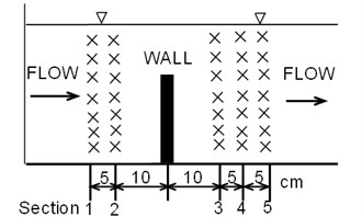
Fig. 2Measured and computed horizontal velocity components at two sections of experiment
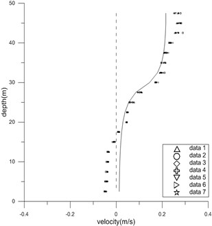
a)
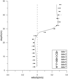
b)
Velocities were measured seven times at every point. Two large vortices were observed at both upstream and downstream, see Fig. 2.
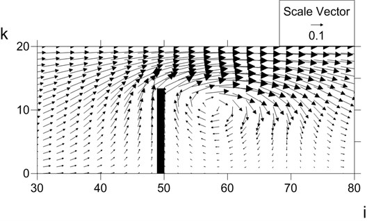
Numerical computation was also carried out with several parameters chosen as: spatial increment in the direction = 2.5 cm, spatial increment in the direction = 2.5 cm, temporal increment = 0.001 s, total channel length = 4 m, and 0.14. Computed flow field is shown in Fig. 3. The vectors in the figure represent current direction and speed. The downstream vortex is outstanding, while the weak upstream vortex is seen on vorticity contours.
Fig. 3Computed current field for experimental conditions: arrows are current vectors
Computed and measured horizontal velocity components are compared in Fig. 2. The largest speed error of the computation is within 6 cm/s, which is satisfactory compared to the strongest current speed of 30 cm/s. The results demonstrates the overall behavior of the numerical model is reasonable.
4. Conclusions
Sigma-coordinate is useful for describing free-surface flows at coasts and rivers. Previous sigma-approaches have solved the Poisson equation on the hydrodynamic pressure, which involves heavy matrix-solving effort. Here computation of hydrodynamic pressure is included in sigma-coordinate approach with the divergence-dispersion method. Equation for divergence on sigma-coordinate is introduced by modifying the existing divergence-dispersion method, SOLA, which is valid for fixed -grid only. The divergence is converted to a difference form, and adopted in a numerical model, CST3D.
The new scheme was validated against a laboratory experiment which is a non-uniform uni-directional flow in a channel. The model is believed to have reproduced experimental results well. The present modified SOLA could expand its usage for more general geometry or structure in the future.
References
-
Tetra Tech Inc. The Environmental Fluid Dynamics Code: Theory and Computation Volume 1: Hydrodynamics and Mass Transport. US EPA Version 1.01, 2007.
-
Delft Deltares. Delft3d-Flow: Simulation of Multi-Dimensional Hydrodynamic Flows and Transport Phenomena Including Sediments: User Manual: Hydro-Morphodynamics: Version 3.15.33641, 2014.
-
DHI. Mike21 & Mike3 Flow Model FM: Hydrodynamic Module: Short Description. Horsholm, DHI, 2013.
-
Ho D., Boyes K., Donohoo S., Cooper B. Numerical flow analysis for spillways. Proceedings of the 43rd ANCOLD Conference, Hobart, Tasmania, 2003, p. 1-11.
-
ANSYS Inc 2012 ANSYS FLUENT. Theory Guide: Release 14.5. Canonsburg: ANSIS.
-
Lin P. A multiple-layer sigma-coordinate model for simulation of wave-structure interaction. Computer and Fluids, Vol. 35, 2006, p. 147-167.
-
Keilegavlen E., Berntsen J. Non-hydrostatic pressure in σ-coordinate ocean models. Ocean Modelling, Vol. 28, 2009, p. 240-249.
-
Zhu L., Chen Q., Wan X. Numerical modeling of nonlinear water waves with sigma coordinate and layer thickness optimization. Proc. XIX Int. Conference on Water Resources, University of Illinois at Urbana-Champaign, 2012.
-
Hirt C. W., Nichols B. D., Romero N. C. SOLA: A numerical solution algorithm for transient fluid flows. Los Alamos, Los Alamos Scientific Lab, 1975.
-
Jang C., Kim H., Lim N. A development of coupled wave-induced current modeling system and its application to the idealized shoreline with detached breakwater. Journal of Wetlands Research, Vol. 14, 2012, p. 439-455, (in Korean).
-
Kim H. Coastal sediment transport prediction model (CST3D): Version 2013-v1: User manual. Seoul, Saerom, 2013, (in Korean).
About this article
This includes research results of “MIDAS” 2014, and “MEPS” 2013 supported by Ministry of Oceans and Fisheries (Korea).
