Inspection period determination for two-stage degraded system

Ni, Xianglong; Zhao, Jianmin; Zhang, Xinghui; Wang, Zhe

Vibroengineering Procedia

Browse Procedia

Published: 03 November 2014

Check for updates

Inspection period determination for two-stage degraded system

Xianglong Ni¹

Jianmin Zhao²

Xinghui Zhang³

Zhe Wang⁴

^{1, 2, 3, 4}Mechanical Engineering College, Shijiazhuang, China

Corresponding Author:

Xianglong Ni

Cite the article Download PDF

Downloads 1254

Abstract

At present studies on degradation process are mainly single stage degradation mode, however, in practice the system degradation process is generally multi-stage. Based on general degradation process modeling, the paper assumed degenerate distribution of two-stage mode obey various normal distribution, shock times obey Poisson process. Reliability modeling and mean time to failure modeling of two-stage degraded mode are studied. Functional check period determination methods are used to calculate inspection periods for different degradation stage. In numerical example, inspection periods for system with two-stage degradation process are analyzed.

1. Introduction

It is impossible to spend a large number of samples for life test in high-tech field. In this case, it is difficult to analyze system reliability using traditional methods. While the most important advantage of degradation modeling is the ability to record multiple degradation data of each individual unit, so obtaining failure data there does not need to wait for fault [1]. Therefore, performance degradation data is uesd to analyze system reliability and inspection period [2].

In literature [3-5] existing degradation failure analysis methods which were mainly single-stage mode for system degradation process were well summarized. In practice, the degradation process is often multi-stage and different degradation stages obey different distributions.

The objective of this paper is to study the degradation characteristic of system with two-stage degraded mode. In section 2 degradation process principle is expounded. In section 3 reliability and modeling methods for mean time are mentioned. Section 4 functional mainly researches methods of check period determination. In section 5, a numerical example is presented to illustrate inspection periods for different system degradation stage.

2. Degradation process principle

When system is operating or in used, stress suffered causes damage to the system, and damage gradually accumulate. The damage accumulation leads to system performance degradation. While damage accumulation caps a certain level the system will fault. With the system performance decline, the system produces relevant condition parameters which can characterize system degradation degree. Beyond that those condition parameters provide key information to assess system reliability and health condition [6].

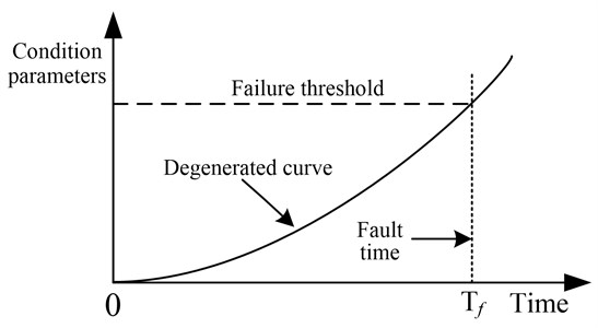
With system degrading, some performance parameters appear trending change, when the parameters reach a pre-specified threshold while the system performance can not meet the prescribed requirements, we can consider that the system failure. As shown in Fig. 1, within time $[0, T_{f}]$ condition parameters present gradually increasing trend, but condition parameters do not meet the prescribed requirements, so the system is in normal working condition. While in time $[T_{f}, \infty]$ , the condition parameters exceed failure threshold, so it can be regarded as that the system is fault. $T_{f}$ is fault time.

Fig. 1Cumulative degradation process

3. Determination modeling for two-stage mode

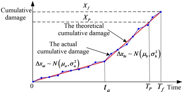
System degradation process with two-stage is shown in Fig. 2 [7]. In system degradation process, at time $t_{a}$ the deterioration rate has a sudden change which duing to the internal mechanism or external environment influences. $t_{a}$ is the connection time point for the first and second stage. In first stage the system deterioration rate in line with the normal distribution $Δ x_{a i} ~ N (μ_{a}, σ_{a}^{2})$ while in second stage it is $Δ x_{b i} ~ N (μ_{b}, σ_{b}^{2})$ . $X_{f}$ is the cumulative damage failure threshold, $T_{f}$ is the time point that system cumulative damage reach the failure threshold, that is system life. $X_{p}$ is the cumulative damage alarm threshold, $T_{p}$ is the time point when system cumulative damage reaches alarm threshold. Shock damage between the first stage and the second stage are unrelated and each shock damage is independent and random process in all system life [ $0, T_{f}$ ].

Fig. 2System cumulative damage for two-stage mode

3.1. Cumulative damage

Suggest that $\{t_{i}; i = 0, 1, 2, 3,..., n\}$ are shock time series, and $t_{0} = 0;$ $\{Δ x_{i}; i = 0, 1, 2, 3,..., n\}$ are damage amount caused by shocks, and the system is working well at beginning, namely initial damage amount $Δ x_{0} = 0$ assuming $Δ x_{0}$ is independent identically distributed and independently from $t_{i}$ . The shock damage time $t_{c}$ may in the first stage ( $0 \leq t_{c} \leq t_{a}$ ) or the second stage ( $t_{a} < t_{c} \leq T_{f}$ ). Different values for $t_{c}$ make different cumulative damage calculation methods. Random variable $\{N_{c}; t_{c} \geq 0\}$ represents the total number of shock times within time $[0, t_{c}]$ .

When $0 \leq t_{c} \leq t_{a}$ , the cumulative damage is:

1

x_{c} = \sum_{i = 1}^{N_{c}} Δ x_{a i}, N_{c} = 1, 2, \dots .

Assuming that damaged frequence of system caused by shocking obey Poisson distrbution. From the Poisson process theoretical we can know that the probability of shock times just as $n$ within time $[0, t_{c}]$ is:

2

P (N_{c} = n) = \frac{{(λ t)}^{n}}{n!} e^{- λ t} .

When $t_{a} < t_{c} \leq t_{f}$ , system cumulative damage makes up by damage in the first stage and the second stage. Shock damage time in the first stage is $t_{a}$ , while $t_{c} - t_{a}$ in the second stage. System cumulative damage is:

3

x_{c} = \sum_{i = 1}^{N_{a}} Δ x_{a i} + \sum_{j = 1}^{N_{b}} Δ x_{b j}, N_{a}, N_{b} = 1, 2, \dots,

where $N_{a}, N_{b}$ are respectively represent the shock damage times of system in first stage and second stage.

As every shock damage is independently and unrelated, so $\sum_{i = 1}^{N_{a}} Δ x_{a i} ~ N (N_{a} μ_{a}, N_{a} σ_{a}^{2}),$ $\sum_{i = 1}^{N_{b}} Δ x_{b i} ~ N (N_{b} μ_{b}, N_{b} σ_{b}^{2})$ , and:

4

\sum_{i = 1}^{N_{a}} Δ x_{a i} + \sum_{i = 1}^{N_{b}} Δ x_{b i} ~ N (N_{a} μ_{a} + N_{b} μ_{b}, N_{a} σ_{a}^{2} + N_{b} σ_{b}^{2}) .

Shocks between the two stages are independently, there is:

5

P (N_{a} = m, N_{b} = n) = P (N_{a} = m) P (N_{b} = n) = \frac{{(λ t_{a})}^{m}}{m!} \cdot \frac{{[λ (t_{c} - t_{a})]}^{n}}{n!} \cdot e^{- λ t_{c}} .

3.2. System reliability

System reliability refers to the probability for system cumulative damage $x_{c}$ less than cumulative damage failure threshold $X_{f}$ when shock time is $t_{c}$ .

When $0 \leq t_{c} \leq t_{a}$ , system reliability is:

6

\begin{matrix} R_{1} (t) = P (x_{c} \leq X_{f}) = \sum_{n = 1}^{\infty} P (\sum_{i = 1}^{N_{a}} Δ x_{a i} \leq X_{f}| N_{a} = n) \cdot P (N_{a} = n) \end{matrix}

= \sum_{n = 1}^{\infty} P (\sum_{i = 1}^{n} \frac{Δ x_{a i} - μ_{a}}{\sqrt{n} σ_{a}} \leq \frac{X_{f} - n μ_{a}}{\sqrt{n} σ_{a}}) \cdot P (N_{a} = n) = \sum_{n = 1}^{\infty} Φ (\frac{X_{f} - n μ_{a}}{\sqrt{n} σ_{a}}) \cdot \frac{{(λ t_{c})}^{n}}{n!} \cdot e^{- λ t_{c}} .

If system degradation process is traditional single stage degradation mode, the system reliability is Eq. (6) either.

When $t_{a} < t_{c} \leq T_{f}$ , system cumulative shock time is $t_{c} - t_{a}$ in the second stage, system reliability is:

7

R_{2} (t) = P (x_{c} \leq X_{f}) = P (\sum_{i = 1}^{N_{a}} Δ x_{a i} + \sum_{i = 1}^{N_{b}} Δ x_{b i} < X_{f})

= \sum_{m = 1}^{\infty} \sum_{n = 1}^{\infty} P (\sum_{i = 0}^{m} Δ x_{a i} + \sum_{i = 0}^{n} Δ x_{b i} < X_{f}) \cdot P (N_{a} = m, N_{b} = n)

= \sum_{m = 1}^{\infty} \sum_{n = 1}^{\infty} Φ (\frac{X_{f} - (m μ_{a} + n μ_{b})}{\sqrt{m σ_{a}^{2} + n σ_{b}^{2}}}) \cdot P (N_{a} = m) \cdot P (N_{b} = n)

= \sum_{m = 1}^{\infty} \sum_{n = 1}^{\infty} Φ (\frac{X_{f} - (m μ_{a} + n μ_{b})}{\sqrt{m σ_{a}^{2} + n σ_{b}^{2}}}) \cdot \frac{{(λ t_{a})}^{m}}{m!} \cdot \frac{{[λ (t - t_{a})]}^{n}}{n!} \cdot e^{- λ t} .

3.3. Mean time to failure

If the system degradation process is traditional single stage degradation mode, mean time to failure of the system is:

8

M_{1} (t) = \int_{0}^{\infty} R_{1} (t) d t = \int_{0}^{\infty} (\sum_{n = 1}^{\infty} Φ (\frac{X_{f} - n μ_{a}}{\sqrt{n} σ_{a}}) \cdot \frac{{(λ t)}^{n}}{n!} \cdot e^{- λ t}) d t = \frac{1}{λ} \sum_{n = 1}^{\infty} Φ (\frac{X_{f} - n μ_{a}}{\sqrt{n} σ_{a}}) .

In system degradation with two stage mode the system fault occurres in the second stage. System life $T_{f}$ is affected by shock strength $Δ x_{a i}$ , $Δ x_{b i}$ and shock time $t_{a}$ for the first stage. The mean time to failure of the system is:

9

M_{2} (t) = \int_{t_{a}}^{\infty} R_{2} (t) d t

= \int_{t_{a}}^{\infty} (\sum_{m = 0}^{\infty} \sum_{n = 0}^{\infty} Φ (\frac{x_{f} - (m μ_{a} + n μ_{b})}{\sqrt{m σ_{a}^{2} + n σ_{b}^{2}}}) \cdot \frac{{(λ t_{a})}^{m}}{m!} \cdot \frac{{[λ (t - t_{a})]}^{n}}{n!} e^{- λ t}) d t

= \sum_{m = 0}^{\infty} \sum_{n = 0}^{\infty} Φ (\frac{x_{f} - (m μ_{a} + n μ_{b})}{\sqrt{m σ_{a}^{2} + n σ_{b}^{2}}}) \cdot \frac{{(λ t_{a})}^{m}}{m!} e^{- λ t_{a}} \cdot \int_{t_{a}}^{\infty} (\frac{{(λ (t - t_{a}))}^{n}}{n!} e^{- λ (t - t_{a})}) d t

= \sum_{m = 0}^{\infty} \sum_{n = 0}^{\infty} Φ (\frac{x_{f} - (m μ_{a} + n μ_{b})}{\sqrt{m σ_{a}^{2} + n σ_{b}^{2}}}) \cdot \frac{{(λ t_{a})}^{m}}{m!} e^{- λ t_{a}}

\cdot \{\frac{1}{λ} \cdot \int_{0}^{\infty} (\frac{{(λ (t - t_{a}))}^{n}}{n!} e^{- λ (t - t_{a})}) d (λ (t - t_{a}))\}

= \frac{1}{λ} \cdot \sum_{m = 0}^{\infty} \sum_{n = 0}^{\infty} Φ (\frac{x_{f} - (m μ_{a} + n μ_{b})}{\sqrt{m σ_{a}^{2} + n σ_{b}^{2}}}) \cdot \frac{{(λ t_{a})}^{m}}{m!} e^{- λ t_{a}} .

4. Functional check period determination

4.1. P-F process time determination

Suppose the $T_{f}$ is the average life expectancy while cumulative damage is $X_{f}$ , $T_{p}$ is the average life expectancy while cumulative damage is $X_{P}$ . The total time $T_{B}$ from potential failure to function failure (P-F process) is:

10

T_{B} = T_{f} - T_{p},

where $T_{f}$ and $T_{p}$ can be obtained from mean life to failure Eq. (8) and (9).

4.2. Inspection period determination

It is necessary to carry out regular function inspection for a system with safety and task influence. Assumes that the acceptable probability of failure with safety or task influence is $F$ , inspection times during $T_{B}$ of P-F process is $k$ , there is:

11

F = {(1 - P)}^{k},

12

k = \frac{l g F}{l g (1 - P)},

where $P$ is fault detection probability for one inspection work.

Inspection period $T$ is:

13

T = \frac{T_{B}}{k} .

5. Numerical example

Degradation process of a system presents two-stage mode as using environment changed. Now the related parameters are beginning to study.

5.1. Parameters estimation

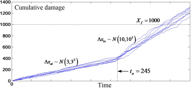
According to system characteristics and application environment, it can be found that failure threshold $X_{f} =$ 1000 and connection time point for the first and second stage $t_{a} =$ 245 h. 8 groups of degradation data were gained from system monitoring before (as shown in Fig. 3). Data is statistics analyzed and obtained degradation parameters. The shock damage for the first stage and the second stage is respectively obeying normal distribution $Δ x_{a i} ~ N (3, 3^{2})$ and $Δ x_{b i} ~ N (10,1 0^{2})$ . The Poisson strength of shock times within $[0, t_{c}]$ is $λ = 0.5$ .

Fig. 3Degradation data and cumulative damage

5.2. Inspection period determination

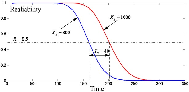
Duing to the system failure threshold $X_{f} = 1000$ , the system cumulative damage alarm $X_{p} = 0.8 X_{f} = 800.$ Take shock damage $Δ x = Δ x_{b i} ~ N (10, 1 0^{2}),$ reliability distribution for $x = X_{p}$ and $x = X_{f}$ were obtained as shown in Fig. 4. Take $R =$ 0.5 as baseline, get the corresponding time points $T_{p}^{b}$ , $T_{f}^{b}$ , so the total time of P-F process is $T_{B}^{b} = T_{f}^{b} - T_{p}^{b} =$ 40 h. Similarly, the total time of P-F process for shock damage $Δ x = Δ x_{a i} ~ N (3, 3^{2})$ is $T_{B}^{a} =$ 110 h.

Fig. 4The reliability distribution for the second stage

Stipulated the acceptable probability of failure with task influence is $F =$ 0.1, fault detection probability for one inspection is $P =$ 0.7. According to Eq. (12) the inspection times during $T_{B}$ is $k =$ 1.9124.

Rounding $k$ get $k = 2$ . Inspection period $T$ can be obtained by Eq. (13):

Inspection periods for the first stage $T_{a} = T_{B}^{a} / k =$ 55 h.

Inspection periods for the second stage $T_{b} = T_{B}^{b} / k =$ 20 h.

Obviously in system with multi-stage degradation mode, inspection periods are different as degradation speed differ from each stage.

6. Conclusions

This paper puts forward degradation modeling methods for system with two-stage degraded mode. Modeling methods of reliability and mean time to failure are studied owing to their importance for prognostics and system health management. Conclusion of this paper shows that inspection periods should be different in different degraded stage. The related theory of system with two-stage degraded mode is enriched in this paper.

References

Zhang Y. Q., Feng J., Liu Q., et al. Reliability analysis based on performance degradation model of compound Poisson-Normal process. Systems Engineering and Electronics, Vol. 28, Issue 11, 2006, p. 1775-1778.

Search CrossRef
Joseph L. C., Meeker W. Q. Using degradation measurements to estimate a time to failure distribution. Technometrics, Vol. 35, Issue 2, 1993, p. 161-174.

Search CrossRef
Couallier V. Some recent results on joint degradation and failure time modeling. Probability, Statistics and Modeling in Public Health, New York, 2006.

Search CrossRef
Deng A. M., Chen X., Zhang C. H., et al. Reliability assessment based on performance degradation data. Journal of Astronautics, Vol. 27, Issue 3, 2006, p. 546-552.

Search CrossRef
Chen L., Hu C. H. Review of reliability analysis methods based on degradation modeling. Control and Decision, Vol. 24, Issue 9, 2009, p. 1281-1287.

Search CrossRef
Nair V. N. Discussion of estimation of reliability in field performance studies by J. D Kalbfleisch and J. F. Lawless. Technometrics, Vol. 30, Issue 4, 1988, p. 379-383.

Search CrossRef
Ni X. L., Zhao J. M., Zhang X. H., et al. System degradation process modeling for two-stage degraded mode. Prognostics and System Health Management Conference, Zhangjiajie, 2014.

Search CrossRef

About this article

Received

Accepted

05 October 2014

Published

03 November 2014

Keywords

degradation modeling

two-stage mode

mean time to failure

inspection period

This is an open access article distributed under the Creative Commons Attribution License, which permits unrestricted use, distribution, and reproduction in any medium, provided the original work is properly cited.