Abstract
The paper proposes the Detrended Fluctuation Analysis (DFA) of the vibration signal for diagnosing of mechanical defects of the vehicle powertrain. The DFA allows investigations of the observed signals with regard to their multifractality. The results of vibration signal analysis of the engine with the damaged exhaust valve and with the unsuitable exhaust valve clearance are presented. During road test the acceleration vibration signal was recorded with additional signals for synchronization and engine timing. The vibration data are analysed by DFA and the resultant scaling-law curve with crossover points are obtained. The estimated Hurst exponents are used in the selection procedure of diagnostic features.
1. Introduction
Vibration signals recorded by acceleration sensors in the vehicle powertrain, during its operation, are characterised by increases of non-stationary and non-linear disturbances caused by wearing out as well as by defects. These systems have periodical properties due to periodical excitations, however it is often difficult to determine the upper time scale or lower limitation of the observation frequency. Such system dynamics can be analysed based on power-law and scaling equations for theoretically unlimited ranges of time or frequency scales and on multifractal models of observed signals.
The self-organising criticality (SOC) theory, inspired by fractality of dynamic systems, arguments that the state of the complex non-linear system is time variable approaching the critical state, in which an arbitrary small parameter change causes a large change in the system. An occurrence of new features not resulting from properties of components of complex systems, called emergency allows for further functioning of the system. This means that the system – by means of the evolution – reveals adaptation abilities forced by its surroundings or by the control system.
Curves of the system scaling-law are changing during operations. It turns out that multifractal exponents present the evolution of features of the complex dynamic system as a function of the operation time.
The dimension of the curve, being the considered signal diagram, is assumed the fractal dimension [1]. The fractal dimension of the time series determines its local roughness. If is the minimal number of circles of dimension , covering the given time series, then . From that:
Self-similar time series or time series exhibiting self-similarity after the integration describe multifractal dimensions , corresponding to Hurst exponents [2], for various scaling ranges, according to the dependency:
Methods of the Detrended Fluctuation Analyses (DFA) [3] and its multifractal version (MF-DFA) [4] can be used as a means of estimating the Hurst exponent. The MF-DFA allowing investigations of the observed signals with regard to their multifractality, assures more stable approach to the multifractal formalism than the previously applied method of the wavelet transform of module maximum (WTMM).
Analytical methods of detrended fluctuations were lately used in the vibroacoustic diagnostics of rotating systems [5] presented the technique of the defects detection of a toothed gear by means of the vector formed from the function of the vibration signals fluctuation and the principal components analysis (PCA). Two methods of standards identification were applied in the work of [6]: the PCA and neural networks technique in relation to the compressed data obtained from the monitoring of bearings operating at various loads and rotational speeds. The data compressing was performed by means of the Rescaled Range (R/S) analysis and DFA. Another way of the monitoring of bearings can be found in the paper [7], where diagnostic features of defects were defined on the bases of the spectrum parameters of the multifractal vibrations signal obtained as the result of the MF-DFA algorithm. [8] proposed also the detection of bearings and toothed gears defects on the bases of the Hurst exponents determined in various scaling ranges of the curves of vibration signals fluctuations.
2. The MF-DFA method
This method is based on the trend elimination from the investigated time series. The procedure is realised in five steps, leading to the Hurst exponent estimation, followed by the multifractal spectrum.
Let it be assumed that the observed time series contains samples.
Step 1. Let’s define the accumulated, centred random variable of the form:
where is the expected value estimator of the time series .
Step 2. Let’s divide the time series into non-overlapping segments of length , starting this division once from the beginning and for the second time from the end. In this way we obtain segments .
Step 3. By the method of least squares for each segment the profile represented by the -th degree will be determined and detrending performed:
for and:
for .
Step 4. Calculated variances are averaged for all segments and the fluctuation functions of the order , are determined:
For we obtain dependency defining fluctuations in the DFA method.
Step 5. After repeating steps 2 to 4 for various time scales , we obtain the power fluctuation dependency:
where is the generalised Hurst exponent.
The statistically reliable estimation of exponents requires the scale selection within limits . The improvement of the estimation accuracy for anti-persistent signals, of the Hurst exponents values being near zero, enables integration of the time series before starting the MF-DFA procedure. Double integration leads to obtaining the exponents of the fluctuation function of values increased by 1, i.e. .
The exponent for monofractals, while it is a decreasing function for multifractals. The fluctuation curve in the log/log scale allows to determine the Hurst exponents and the multifractal spectrum (singular spectrum):
while the singular exponent :
For , MF-DFA is equivalent to DFA and .
3. Description of examinations
Examinations were performed during road tests on the four-cylinder engine of spark ignition of Fiat Punto 1.4 of 400 000 km. mileage. Series of engine vibration measurements for various rotational speeds and loads were performed. The main measuring path included the piezoelectric vibration sensors B&K Delta Shear type 4393 of a frequency range: 0.1 – 16500 Hz, resonance frequency 55 kHz and work temperatures from –74 to +250oC, fastened by means of a joint screwed into the engine side at cylinder 1, and the portable device for recording data B&K PULSE type 3560E. Accelerations of engine block vibrations were recorded in the vertical and horizontal directions with a frequency of 65536 Hz. Then the signal was pre-processed with antialiasing filter to avoid amplifying the components in the natural frequency band of the vibration sensor.
Apart from the engine vibrations signal also the crankshaft position signal, throttle position and signals from the ignition coil at 1 and 4 cylinder were recorded. Additional signals enabled the identification of engine working cycles, injection moments, ignition and timing of gear phases. Signals of 1-minute duration were recorded during driving with a constant speed. Small speed fluctuations were eliminated during further analysis. Maintaining the constant rotational speed of the engine is essential, since this parameter has a significant influence on the vibration amplitude. A load influence is not as important as speed. The vibration signal was resampled in order to equalise the number of samples analysed in each cycle of engine operations. This procedure enabled changing the domain from the time into the angle of rotation of the crankshaft, during the analysis.
Examinations were performed for various maintenance states of the exhaust valve [9]:
• Valve in a good working order, optimal clearance (0.25 mm),
• Valve in a good working order, increased clearance (+0.06 mm),
• Valve in a good working order, decreased clearance (–0.06 mm),
• Valve out of order I (small defect), optimal clearance,
• Valve out of order II (large defect), optimal clearance.
Valve defect I constituted the valve head cut 3 mm long, while defect II had this cut increased to 6 mm. Instantaneous time progresses of the acceleration of vibrations for various maintenance states are presented in Figure 1.
Fig. 1Time series – engine head vibrations at 3000 rpm for one work cycle of engine: a) valve in a good working order, optimal clearance (0.25 mm), b) valve in a good working order, increased clearance (+0.06 mm), c) valve in a good working order, decreased clearance (–0.06 mm), d) valve out of order I (small defect), optimal clearance, e) valve out of order II (large defect), optimal clearance
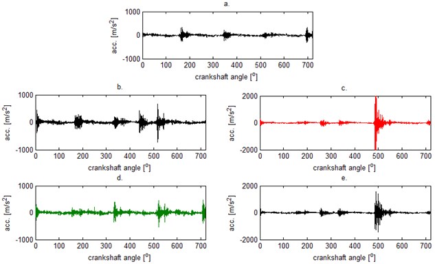
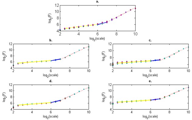
Fig. 2Fluctuation versus the segment (scale) for: a) valve in a good working order, optimal clearance (0.25 mm), b) valve in a good working order, increased clearance (+0.06 mm), c) valve in a good working order, decreased clearance (-0.06 mm), d) valve out of order I (small defect), optimal clearance, e) valve out of order II (large defect), optimal clearance
4. Further analyses
The integrated time series of a length of two work cycles of the engine (7200 samples) were divided into segments of the same length. In each segment the linear trend was determined and then removed. Next, the RMS fluctuation of the trendless integrated time series was determined from equation (6). It was performed for the set of time scales s of the length from 4 to 1024 samples, to obtain the time independent measure. The connection between the average fluctuation and the segment (scale) size for the tested cases of the exhaust valve defects, were determined for 30 time series and are presented in Figure 2.
The Hurst exponent is defined as an inclination of curve in the double logarithmic diagram. In order to determine this exponent the approximation of curves by straight lines for three scale ranges: 6 – 64, 64 – 128, 128 – 1024 was performed. The average Hurst exponents for the tested cases are listed in Table 1.
Table 1Average Hurst exponent in segments for tested defects of valve
Good valve | Defected (small) | Defected (big) | Decreased clearance | Increased clearance | |
Hurst exponent 1 scale: 6 – 64 | 0.365 | 0.234 | 0.188 | 0.245 | 0.185 |
Hurst exponent 2 scale: 64 – 128 | 0.711 | 0.688 | 0.406 | 0.519 | 0.301 |
Hurst exponent 3 scale: 128 – 1024 | 1.497 | 1.424 | 1.324 | 1.450 | 1.319 |
The first singled out scale range is characterised by the inclination coefficient: 0 < < 0.5, which means long-range anti-correlations. The second scale range of the inclination coefficient: 0.5 < <1 indicates occurring of long-range power-law correlations, however as the defect grows the coefficient falls below 0.5. In the third range the inclination coefficient > 1 indicates the correlation occurrence but not of a power-law character. It is the result of the occurrence of harmonic components originated from driving shafts and cylinders operations.
The Hurst exponent was listed versus the Hurst exponent in Figure 3. The data were classified by the nearest neighbour method for 30 other time series for the tested cases of defects and the instantaneous Hurst exponent was shown at the background of average exponents from Table 1.
Fig. 3The classification of the classified maintenance states using the first and second Hurst exponent
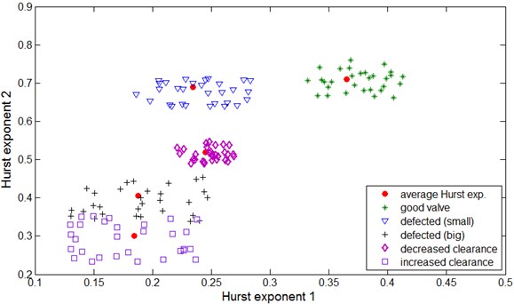
The following remarks can be drawn from the Figure 3 analysis:
• As the exhaust valve defect increases the Hurst exponents and decrease.
• The method allows to detect an initial defect of a valve and decreased valve clearance.
• At a large valve defect and increased valve clearance the areas on the plane are weakly separable and it can happen that – at a certain phase of the defect – they can overlap.
5. Conclusions
The presented example of the application of the detrended fluctuation analysis indicates that this method allows to perform the diagnostics of the exhaust valve defects of I.C. engines and the wrong valve clearance. After determining the Hurst exponents in single segments it was possible to separate areas related to individual defects on the plane also for initial defects. It is planned to apply generalized Hurst exponents and the singularity spectrum based analysis in further studies. The classification by the nearest neighbour method will be performed.
References
-
Butar F. B., Kale M. Fractal analysis of time series and distribution properties of Hurst exponent. Journal of Mathematical Sciences and Mathematics Education, Vol. 6, No. 1, 2011, p. 8-19.
-
Hurst H. E. Long term storage capacity of reservoirs. Transactions of the American Society of Agricultural Engineers, Vol. 116, 1951, p. 770-799.
-
Peng C. K., Havlin S., Stanley H. E., Goldberger A. L. Quantification of scaling exponents and crossover phenomena in nonstationary heartbeat time series. Chaos, Vol. 5, 1995, p. 82-87.
-
Kantelhardt J. W., Zschiegner S. A., Koscielny-Bunde E., Havlin S., Bunde A., Stanley H. E. Multofractal detrended fluctuation analysis of nonstationary time series. Physica A, Vol. 316, 2002, p. 87-114.
-
Moura E. P., Vieira A. P., Irmao M. A. S., Silva A. A. Applications of detrended-fluctuation analysis to gearbox fault diagnosis. Mechanical Systems and Signal Processing, Vol. 23, 2009, p. 682-689.
-
Moura E. P., Souto C. R., Silva A. A., Irmao M. A. S. Evaluation of principal component analysis and neural network performance for bearing fault diagnosis from vibration signal processed by RS and DF analyses. Mechanical Systems and Signal Processing, Vol. 25, 2011, p. 1765-1772.
-
Lin J., Chen Q. Fault diagnosis of rolling bearings based on multifractal detrended fluctuation analysis and Mahalanobis distance criterion. Mechanical Systems and Signal Processing, Vol. 38, 2013, p. 515-533.
-
Lin J., Chen Q. A novel method for feature extraction using crossover characteristics of nonlinear data and its application to fault diagnosis of rotary machinery. Mechanical Systems and Signal Processing, Vol. 48, 2014, p. 174-187.
-
Puchalski A., Komorska I. Application of vibration signal Kalman filtering to fault diagnostics of engine exhaust valve. Journal of Vibroegineering, Vol. 15, Issue 1, 2013, p. 152-158.
About this article
