Optimal design of piezoelectric vibration devices with constrained variable algorithm and FEA

Chen, Ying; Ye, Cui; Kang, Rui

Journal of Vibroengineering

Browse Journal

Submit article

Published: 30 September 2014

Check for updates

Optimal design of piezoelectric vibration devices with constrained variable algorithm and FEA

Ying Chen¹

Cui Ye²

Rui Kang³

^{1, 2, 3}Science and Technology on Reliability and Environmental Engineering Laboratory, Beihang University, Beijing, 100191, P. R. China

Corresponding Author:

Ying Chen

Cite the article Download PDF

Downloads 1066

Abstract

Optimal design of piezoelectric vibration devices used in medical fields is a typical inequality constrained optimization problem. Constrained variable method, as the best algorithm to solve nonlinear constraint optimization problem is used in the optimal design of the piezoelectric devices. The object functions and constrain functions are automatically calculated with Finite Element Analysis software ANSYS, and the results will return to the main optimization program. Results show that compared with the given initial parameters, the vibration amplitude of the optimum piezoelectric vibration device is dramatically increased under the constraint that the stress concentration of the cutting tool is within limit. Experiments are also performed to measure the vibration amplitude. Results are in great agreement with the theoretical one.

1. Introduction

Piezoelectric vibration devices are widely used in cleaning, machining, dental and surgery. When apply in medical field, they must meet the requirements of high output power, high efficiency, lightweight and high reliability [1]. For piezoelectric devices used in bone surgery, the demand of high power and high reliability are incompatible. For example, change of structure is the necessary method to achieve high output power, however this will also lead to stress concentration and increase the probability of device breakage [2-3]. In a word, design of piezoelectric vibration devices is an optimization problem with multi-design variants, multi-constraints and multi-object.

Previous studies of piezoelectric vibration devices optimization are mostly based on electrical equivalent circuit or based on experience of the designers [4-6]. Lockwood etc. [7] describes a method of modelling transducers using network theory, which is determined from measurement of the transducer impedance in water and the pulse-echo response of the system for a given electrical source and load. P. Tierce etc. [8] pointed out that finite-element method is a new way to predict vibratory behaviour and can provide information for optimization of piezoelectric transducers. Pascal [9] proposed a method which integrated finite-element method and some experimental results to study the effects of elementary ceramic rods width-to-thickness ratio.

Among numerous optimization algorithms, Constrained Variable Method is an excellent non-linear constrained optimization method, which was firstly introduced by Wilson in 1963 and consummated by Han in 1977 [10] and Powell in 1978 [11]. This method has the advantage of fast convergence speed, high efficiency, good stability and excellent adaptability. Thus, it has been widely used in engineering applications [12]. Finite Element Analysis (FEA) is widely used in engineering field [13] and can be used to achieve some constraint variable.

In this paper, a new method to optimize piezoelectric vibration devices is proposed. This method integrates Constrained Variable Algorithm with (FEA) method, in which FEA will provide the value of optimization variant, constraint function and object function to the main algorithm program.

The remainder of the paper is organized as follows. Section 2 introduced the theory of Constrained Variable Method. Section 3 describes the proposed optimization method with its flow diagram. Section 4 presents the piezoelectric coupled FEA theory. Section 5 uses an example to illustrate the optimization procedures, and the effectiveness of the proposed methodology.

2. Constrained variable optimization method

An inequality constrained optimization problem can be described as:

1

x = {[x_{1}, x_{2}, \dots \dots, x_{n}]}^{T},

m i n f (x),

s.t. g_{j} (x) \geq 0, j = 1, 2, \dots, m,

{\underline{x}}_{i} \leq x_{i} \leq {\bar{x}}_{i}, i = 1, 2, \dots, n,

where $x$ is design variable vector, $g (x)$ is constrain function and is object function. ${\underline{x}}_{i}$ and ${\bar{x}}_{i}$ are the minimal and maximum limit of design variables.

To solve this optimization problem by constrained variable method, Eq. (1) should firstly convert to its quadratic programming sub-problem, and then looks for the optimal results by Newton iteration method.

The corresponding quadratic programming problem of Eq. (1) is:

2

d = {[d_{1}, d_{2}, \dots \dots, d_{n}]}^{T},

m i n \frac{1}{2} d^{T} B^{k} d + \nabla f {(x^{k})}^{T} d,

s.t. g_{j} (x^{k}) + \nabla g_{j} {(x^{k})}^{T} d \geq 0, j = 1, 2, \dots, m,

{\underline{x}}_{i} \leq x_{i}^{k} + d \leq {\bar{x}}_{i}, i = 1, 2, \dots, n,

where $d$ is search direction, $\nabla f (x^{k})$ and $\nabla g_{j} (x^{k})$ are gradient of object function and constraint functions, $B^{k}$ is revision Hessian Matrix of Lagrange function.

To solve Eq. (2) by Newton method, search direction must be firstly determined. Then search step can be calculated with one-dimensional search method.

Zanggwill penalty function is used as one-dimensional search function, which is:

3

Φ (α) = f (x^{k} + α d^{k}) + \sum_{j = 1}^{m} μ_{j} m a x \{0, - g_{j} (x^{k} + α d^{k})\}

+ \sum_{i = 1}^{n} λ_{i} m a x \{0, x_{i}^{k} + α d^{k} - {\bar{x}}_{i}, {\underline{x}}_{i} - x_{i}^{k} - α d^{k}\},

where $α$ is search step, to increase convergence speed, imprecise search is usually adopted, the searching rule is:

4

Φ (α_{k}) \leq Φ (0) + 0.1 α_{k} Φ^{'} (0),

where $Φ (α)$ is a segment function. Firstly let $α = 1$ , then calculate Eq. (4), if it is not satisfied, let $α$ equal to 0.1, 0.01, … until Eq. (4) is satisfied.

To solve Eq. (1), the derivatives of object function and constraint function to the design variables should be calculated, this process is called characteristic sensitivity analysis. Finite difference method is adopted here to calculate the sensitivity:

5

\frac{\partial u_{i}}{\partial x_{j}} = \frac{u_{i} (x + Δ x_{j}) - u_{i} (x)}{Δ x_{j}}, j = 1, 2, \dots, n,

where $u$ is object function or constraint function, $Δ x_{j}$ is step size, and can be selected by experience.

3. The proposed optimization method

Flow diagram of the proposed optimization method is shown in Fig. 1.

Fig. 1Flow diagram of the proposed optimization method

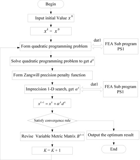
Step 1: Give an initial value $x^{0}$ and convergence accuracy $ε_{1}$ , $ε_{2}$ , let $B^{0} = I$ , $k = 0$ .

Step 2: Call interface subprogram PS1, calculate the constraint function $g (x^{k})$ and object function $f (x^{k})$ with FEA, and also the gradient of constraint function $\nabla g (x^{k})$ and object function $\nabla f (x^{k})$ .

Step 3: Form quadratic programming problem, obtain search direction $d^{k}$ .

Step 4: Perform one-dimensional search, and get $α^{k},$ $x^{k + 1} = x^{k} + α^{k} d^{k},$ call interface subprogram PS1 to calculate $g (x^{k + 1})$ , $f (x^{k + 1})$ , $\nabla g (x^{k + 1})$ and $\nabla f (x^{k + 1})$ .

Step 5: Judge whether the convergence criteria is satisfied. If the answer is yes, optimization result is obtained, otherwise go to step 6.

Step 6: Revise variable metric matrix $B_{k}$ . Let $k = k + 1$ and go to step 3.

The function of interface subprogram PS1 may transmits data between optimization program and ANSYS software via data file called dat1. These data include design variables, constrain variables and object variables.

Dat1 is a batch file programed by ANSYS APDL. The main function of this file includes: (1) Read the design variables, constrain variables and object variables from main program. (2) Parametric modeling and mesh automatically. (3) Loading and solve the problem. (4) Post processing and extract the needed data. (5) Output the constrain variables and object variables to the main program.

4. Piezoelectric coupled FEA theory

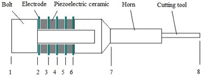
A typical structure of piezoelectric vibration devices is shown in Fig. 2, which mainly includes the bolt, electrode, piezoelectric ceramics, horn and cutting tool. Based on piezoelectric effect, the ceramic convert electric signal into mechanical vibration at the tip of the cutting tool, which vibrates longitudinally to scrape or cut bone.

Fig. 2Typical structure of piezoelectric vibration devices

Assumptions are made in Finite Element Analysis, which are: (1) Thickness of bonding agent between piezoelectric ceramic plates is negligible. (2) Thickness of the electrode slice is negligible compared with piezoelectric ceramic plates. (3) Mechanical friction between piezoelectric ceramic and other parts is negligible. (4) Performance loss of piezoelectric material and other parts is negligible. (5) Piezoelectric material is isotropic, polarization direction is $Z$ axis.

Fundamental equations of piezoelectric vibration devices include constitutive equation, motion equation, geometric equation and boundary conditions.

4.1. Constitutive equation

4.1.1. Piezoelectric constitutive equation

Suppose that the piezoelectric polarization direction, electric field and mechanical vibration direction are all parallel to $Z$ axis. The piezoelectric constitutive equation is:

6

\{\begin{array}{l} D = ε_{s s}^{s} E + e_{s s} S, \\ T = - e_{s s} E + c_{s s}^{E} S, \end{array}

where $T$ , $S$ , $D$ and $E$ are stress vector, strain vector, electrical displacement vector and electrical field intensity vector. $c_{33}^{E}$ is elastic stiffness coefficient under constant electrical field intensity, $e_{33}$ is piezoelectric stress constant and $ε_{33}^{S}$ is material dielectric constant.

4.1.2. Constitutive equation for other parts

Materials of other part of the piezoelectric device are all isotropic linear elastic materials, their constitutive equation is:

7

\{\begin{array}{l} σ_{r} = λ θ + 2 G ε_{r}, \\ σ_{θ} = λ θ + 2 G ε_{θ}, \\ σ_{z} = λ θ + 2 G ε_{z}, \\ τ_{r z} = G γ_{r z}, \end{array}

where $λ$ and $G$ are constant parameters:

8

λ = \frac{E ν}{(1 + ν) (1 - 2 ν)}, G = \frac{E}{2 (1 + ν)},

where $E$ and $ν$ are Young modulus and Poisson’s ratio.

4.2. Motion equation

The basic equation of motion of elasti-mechanics under cylindrical coordinate is:

9

\begin{matrix} \frac{\partial σ_{r}}{\partial r} + \frac{\partial τ_{r z}}{\partial z} + \frac{σ_{r} - σ_{θ}}{r} + F_{r} = ρ \frac{\partial^{2} u_{r}}{\partial t^{2}}, \\ \frac{\partial τ_{r z}}{\partial r} + \frac{\partial σ_{z}}{\partial z} + \frac{τ_{r z}}{r} + F_{z} = ρ \frac{\partial^{2} w}{\partial t^{2}}, \end{matrix}

where $F_{r}$ and $F_{z}$ are body forces of axial direction and $Z$ direction. $u_{r}$ and $w$ are displacement component of axial direction and $Z$ direction.

4.3. Geometric equation

The relationship between stain and displacement of elastic material, which is also called geometric equation, is given under cylindrical coordinate:

10

ε_{r} = \frac{\partial u_{r}}{\partial r}, ε_{θ} = \frac{u_{r}}{r}, ε_{z} = \frac{\partial w}{\partial z}, γ_{r z} = \frac{\partial u_{r}}{\partial z} + \frac{\partial w}{\partial r} .

4.4. Boundary conditions

Boundary at 1 and 8 location (Fig. 2) is free-surface condition; the stress at the surface is zero, i.e. $σ_{i j} n_{i} = 0$ . Boundary of 2, 4 and 6 are electrical free surface, the electric density at electrical charge free surface is zero, which is $D_{i} n_{j} = 0$ . The electric potential at electrical potential free surface is zero, which is $ϕ = 0$ . At boundary of 3 and 5, given electrical charge free surface the electric charge density boundary condition is $D_{i} n_{j} = \bar{w}$ . Given electrical potential free surface the electric potential boundary condition is $ϕ = \bar{ϕ}$ . Location 7 is clamped boundary and $u_{i} = 0$ , $i = x$ , $y$ , $z$ , where $u_{i}$ is the displacement at three axis.

4.5. Finite element method

Constitutive Eq. (6)-(8), motion Eq. (19), geometric Eq. (10) and boundary conditions constitute the governing equation of the piezoelectric device and can be solved by numerical method, such as finite element method.

With shape function, displacement and electric potential difference of an element is:

11

\{u_{c}\} = {[N^{u}]}^{T} \{u\}, V_{c} = {[N^{V}]}^{T} [V],

where ${u_{c}}$ is element displacement vector, $V_{c}$ is element voltage vector, ${u}$ is node displacement matrix, ${V}$ is node electromotive force vector, $[N^{u}]$ is displacement shape function matrix, $[N^{V}]$ is voltage shape function matrix:

12

{[N^{u}]}^{T} = [\begin{matrix} N_{1} & 0 & 0 & \dots & N_{n} & 0 & 0 \\ 0 & N_{1} & 0 & \dots & 0 & N_{n} & 0 \\ 0 & 0 & N_{1} & \dots & 0 & 0 & N_{n} \end{matrix}],

where $N_{i}$ is shape function of node $i$ :

13

{[N^{V}]}^{T} = [\begin{matrix} N_{1} & N_{2} & \dots & N_{n} \end{matrix}] .

Motion equation can convert into linear form:

14

[\begin{matrix} [M_{e}] & [0] \\ [0] & [0] \end{matrix}] \{\begin{matrix} \{\ddot{u}\} \\ \{\ddot{V}\} \end{matrix}\} + [\begin{matrix} [C_{e}] & [0] \\ [0] & [0] \end{matrix}] \{\begin{matrix} \{\dot{u}\} \\ \{\dot{V}\} \end{matrix}\} + [\begin{matrix} [K_{e}] & [K_{e}^{c}] \\ {[K_{e}^{c}]}^{T} & [K_{e}^{d}] \end{matrix}] \{\begin{matrix} \{u\} \\ \{V\} \end{matrix}\} = \{\begin{matrix} \{F_{e}\} \\ \{Q_{e}\} \end{matrix}\},

where $[M_{e}]$ is mass matrix:

15

[M_{e}] = \int_{V_{e}} ρ [N^{u}] {[N^{u}]}^{T} d V,

where $V_{e}$ is the volume of the elastic body, which includes mental material and piezoelectric material, $ρ$ is material density, and $[K_{e}]$ is stiffness matrix:

16

[K_{e}] = \int_{V_{e}} {[B_{u}]}^{T} [C] [B_{u}] d V,

where $[C]$ is elastic constant matrix of materials:

17

[B_{u}] = [\begin{matrix} \frac{\partial}{\partial x} & 0 & 0 \\ 0 & \frac{\partial}{\partial y} & 0 \\ 0 & 0 & \frac{\partial}{\partial z} \\ \frac{\partial}{\partial x} & \frac{\partial}{\partial x} & 0 \\ 0 & \frac{\partial}{\partial y} & \frac{\partial}{\partial z} \\ \frac{\partial}{\partial x} & 0 & \frac{\partial}{\partial z} \end{matrix}] {[N^{u}]}^{T},

where $[C_{e}]$ is damping matrix:

18

[C_{e}] = α [M_{e}] + β [K_{e}],

where $α$ and $β$ are Rayleigh damping constant, $[K_{e}^{d}]$ is dielectric matrix and $[K_{e}^{c}]$ is piezoelectric coupling matrix:

19

[K_{e}^{d}] = - \int_{V_{p}} {[B_{V}]}^{T} [μ] [B_{V}] d V,

where $V_{p}$ is the volume of piezoelectric material, $[μ]$ is dielectric constant matrix of piezoelectric material, and:

20

[B_{V}] = \{\begin{matrix} \frac{\partial}{\partial x} \\ \frac{\partial}{\partial y} \\ \frac{\partial}{\partial z} \end{matrix}\} {[N^{V}]}^{T},

21

[K_{e}^{c}] = \int_{V_{p}} {[B_{u}]}^{T} [e] [B_{V}] d V,

where $[e]$ is piezoelectric matrix.

5. A case study

5.1. Piezoelectric device and FEA modeling

The piezoelectric device in this case study is used in bone surgery, which is shown in Fig. 3.

Fig. 3Structure of the piezoelectric device

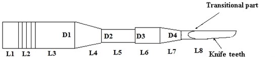
Some of the structure sizes are determined by analytic or empirical calculation, as shown in Table 1.

Table 1Parameters of the structure

Parameters	$L_{1}$	$L_{2}$	$L_{3}$	$L_{5}$	$L_{6}$	$L_{8}$	$D_{1}$	$D_{3}$
Value (mm)	12	12	15	12	9	12	15	$D_{2}$ +3

Other parameters, include $L_{4}$ , $L_{7}$ , $D_{2}$ , $D_{4}$ are design variables. The optimal object is large vibration amplitude at the tip of the cutting tool, and constrain function is the stress at transitional part and the teeth root (shown in Fig. 3) should not exceed their empirical limit, in order to avoid the cutting tool crack due to stress concentration. Thus, the mathematics model of the piezoelectric device optimization problem is given as:

\{x^{*}\} = {\{L_{4}^{*}, L_{7}^{*}, D_{2}^{*}, D_{4}^{*}\}}^{T},

\min f_{1} (x),

s.t.

g_{1} (x) = 1 - \frac{σ_{e q v}^{A}}{[σ_{e q v}^{}]} \geq 0,

g_{2} (x) = 1 - \frac{σ_{e q v}^{B}}{[σ_{e q v}^{}]} \geq 0,

5 \leq L_{4} \leq 8,

3 \leq L_{7} \leq 6,

8 \leq D_{2} \leq 15,

5 \leq D_{4} \leq 12,

where $f_{1} (x)$ is vibration amplitude at the tip of the cutting tool, $g_{1} (x)$ and $g_{2} (x)$ are the constrain functions to avoid crack at transitional part and tooth root. $σ_{e q v}^{A}$ and $σ_{e q v}^{B}$ are the equivalent stress at transitional part and teeth root, $[σ_{e q v}^{}]$ is the empirical stress limit at transitional part and teeth root. $f_{1} (x)$ , $σ_{e q v}^{A}$ and $σ_{e q v}^{B}$ are all calculated by commercial FEA software ANSYS.

In ANSYS, properties of steel, titanium, and PZT8 ceramic are listed in Table 2.

Table 2Material properties

Materials	Young’s modulus (N/m)	Density (kg/m³)	Poisson’s ratio
Steel	2.1×1011	7896	0.29
Titanium	1.05×1011	4450	0.33
PZT8	–	7500	–

Piezoelectric rings are modelled using 3-D coupled-field solid elements SOLID5. The dielectric matrix, piezoelectric matrix (unit: C/m²) and elastic constant matrix (unit: 1010 N/m²) of PZT8 are:

[μ] = [\begin{matrix} 7.97 & 0 & 0 \\ 0 & 7.97 & 0 \\ 0 & 0 & 5.13 \end{matrix}] \times 10^{- 9},

[e] = [\begin{matrix} 0 & 0 & - 4.7 \\ 0 & 0 & - 4.7 \\ 0 & 0 & 12.9 \\ 0 & 10.3 & 0 \\ 10.3 & 0 & 0 \\ 0 & 0 & 0 \end{matrix}],

[c] = [\begin{matrix} 15.6 & 8.86 & 8.45 & 0 & 0 & 0 \\ 15.6 & 8.45 & 0 & 0 & 0 \\ 13.0 & 0 & 0 & 0 \\ 3.13 & 0 & 0 \\ 3.13 & 0 \\ 3.38 \end{matrix}] .

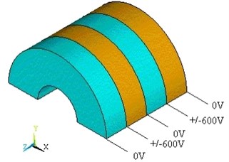
Modal analysis is firstly performed using the Lancoze method. Then harmonic analysis is performed using Sparse Matrix Solver. The input voltage varied sinusoidally between +/–600, which is shown in Fig. 4.

Fig. 4Loads apply on piezoelectric ceramic rings

5.2. Results and discussion

The initial value of design variables $L_{4}$ , $L_{7}$ , $D_{2}$ and $D_{4}$ are 6 mm, 4 mm, 12 mm and 8 mm. After five iterations and call the FEA software 31 times, the optimal results are achieved, which is $L_{4} = 6.78 mm$ , $L_{7} = 3.54 mm$ , $D_{2} = 10.57 mm$ , $D_{4} = 6.26 mm$ .

The values of design variables, constraint functions and object function of each iteration are shown in Table 3.

Table 3Optimization process variables

Parameters	Iteration
Parameters	0	1	2	3	4	5
$L_{4} (mm)$	6.0000	6.2353	6.4172	6.5356	6.7791	6.7833
$L_{7} (mm)$	4.0000	4.0255	3.9828	3.6271	3.5214	3.5421
$D_{2} (mm)$	12.0000	12.1327	11.8201	11.1529	10.6282	10.5719
$D_{4} (mm)$	8.0000	8.0491	7.8934	6.9453	6.3185	6.2624
$g_{1} (x)$	0.1749	0.1828	0.1777	0.1049	0.0732	0.0805
$g_{2} (x)$	0.4371	0.4342	0.4318	0. 4263	0.4256	0.4264
$f_{1} (x) (mm)$	0.0973	0.0939	0.1127	0.1471	0.1482	0.1514

From Table 3, after five iterations, constraint function $g_{1} (x)$ is close to zero, that means the design variables cannot adjust otherwise $g_{1} (x)$ will be negative and violates the constraint condition, and that point is the optimal results. At the beginning, $f_{1} (x)$ is 97.3 um, after the iteration $f_{1} (x)$ is 151.4 um, the optimization object is achieved.

After optimization, equivalent stress distribution of the cutting tool is relatively poorer compared with that of initial value. With initial design variant, the maximum equivalent stress at the cutting tool is 17.7 MPa, while after optimization, this value is 19.0 MPa.

Fig. 5Equivalent stress distribution before and after optimization: a) before optimization, b) after optimization

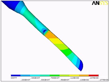
a)

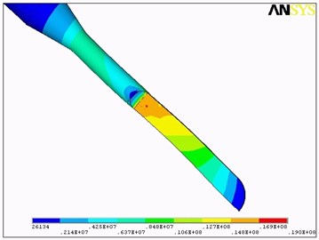
b)

Piezoelectric vibration devices with optimum design parameters is manufactured and assembled, which is shown in Fig. 6.

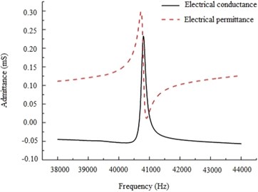
Admittance measurement is carried out with dynamic signal analysis instrument SR785. Results in Fig. 7 show that the resonance frequency of this device is 40.382 kHz. The value is 40.350 kHz in FEA analysis.

Fig. 6Piezoelectric vibration devices with optimum design parameters

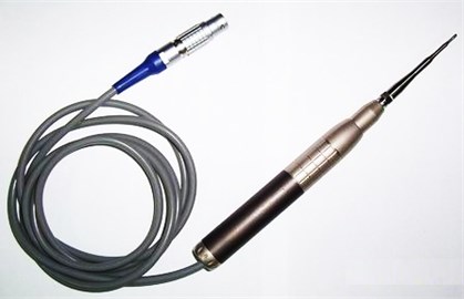
Fig. 7Measurement of resonance frequency of the optimal piezoelectric device

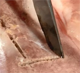
Vibration amplitude of the piezoelectric device is measured with two methods. One is high-speed imaging method with Keyence VHX-100 digital microscope. Fig. 8 shows the schematic diagram of this measurement scheme. The measurement system is composed of a microscope with high-speed digital camera lens, which can pick up the image when piezoelectric device vibrates with ultrasonic frequency.

Fig. 9 shows the images taking with high-speed microscope, where one grid of the scale represents 100 µm. In Fig. 6(b), the vibration belt shows that displacement of the tip is one and a half grids, which is nearly 150 µm.

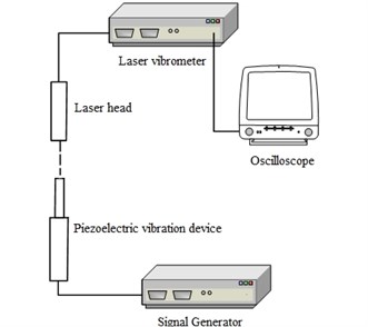
Vibration amplitude measured with high-speed imaging instrument is an approximate value, precise measurement can be achieved by laser Doppler vibrometer, which is shown in Fig. 10. This measurement system is composed of laser Doppler vibrometer (CV700), oscilloscope, and piezoelectric signal generator.

Fig. 8Measurement of tip displacement with high-speed imaging instrument

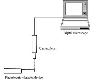
Fig. 9Image of the cutting tool of piezoelectric device: a) resting and b) vibrating condition

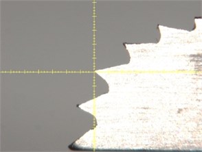
a)

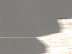
b)

Output signal in Fig. 10 is vibration velocity, which will be integrated to obtain vibration displacement. Fig. 11 shows the vibration displacement at the tip of the piezoelectric device cutting tool, from which the vibration amplitude can be precisely measured, and the results is also near 150 um, consistent with the FEA method and imaging method.

Fig. 10Measurement of tip displacement with laser Doppler vibrometer

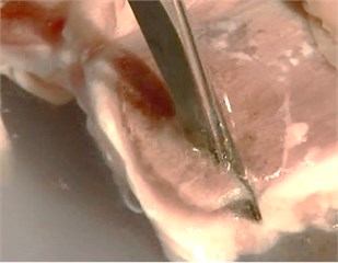
The optimized piezoelectric tool is used to cut different kinds of bones, which is shown in Fig. 12. Spongy bone is from the vertebra and compact bone is from the femur of a pig. The speed when cutting spongy bone is nearly 0.01 m/s, while the speed when cutting compact bone is slightly slower than cutting spongy bone. More than 30 clinical cases also show that the cutting speed of the optimized piezoelectric tool is higher than tradition electric bone grinding tool.

Fig. 11Vibration displacement of cutting tool tip

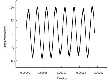
Fig. 12Cutting different bone tissues with optimized piezoelectric tool: a) spongy bone, b) compact bone

a)

b)

Lifetime of 85 piezoelectric bone tools that used in clinical cases are recorded, among these tools, 60 of them are optimized with constrained variable algorithm and FEA method, others are designed with traditional method or by experience of the designer. It is shown in Table 4, lifetime of the optimized tools are longer than those tools that not been optimized.

Table 4Lifetime of piezoelectric bone with and without design optimization

Lifetime (h)	$1 < T \leq 30$	$30 < T \leq 50$	$50 < T \leq 100$	$T > 100$	Total	Average lifetime (h)
Tools with design optimization	1	8	29	22	60	≈80
Tools without design optimization	1	9	10	5	25	≈65

From the above analysis and experiments, the optimized piezoelectric tool can output higher energy, and more efficient in cutting bone, which means doctors will save labour and time to finish the surgery. Although local stress on the tool will increase, lifetime of piezoelectric tools is somewhat improved due to the shape optimization. Conclusions can be drawn that the optimization method with Constrained Variable Algorithm and FEA is very effective to design a high performance piezoelectric surgery tool.

6. Conclusions

Constrained Variable Algorithm and FEA method are used for the optimization of piezoelectric vibration device. Results show that for nonlinear optimization problem with multi-design variants and multi-constraints, Constrained Variable Algorithm has fast convergence speed. And when this algorithm used in engineering fields, FEA software is a good supplement for calculating constraint function and object function.

References

Dong Sun, Zhaoying Zhou, Liu Y. H., Shen Z. Development and application of ultrasonic surgical instruments. Transactions on Biomedical Engineering, Vol. 44, Issue 6, 1997, p. 462-467.

Search CrossRef
Ying Chen, Zhou Z. Y. Effects of different tissue loads on high power ultrasonic surgery scalpel. Ultrasound in Medicine and Biology, Vol. 32, Issue 3, 2006, p. 415-420.

Search CrossRef
Ying Chen, Rui Kang Design for reliability of ultrasonic bone knife. Advanced Science Letters, Vol. 4, Issue 6-7, 2011, p. 2147-2151.

Search CrossRef
Gu Yujiong, Zhou Zhaoying, Yao Jian Ultrasonic vibration system four terminal network method and its application. Chinese Journal of Mechanical Engineering, Vol. 33, Issue 3, 1997, p. 94-101.

Search CrossRef
Sergio S. Design of an optimized high-power ultrasonic transducer. Muhlen Ultrasonics Symposium, 1990, p. 1631-1633.

Search CrossRef
Eisner E., Seager J. S. A longitudinally resonant stub for vibrations of large amplitude. Ultrasonics, 1965, p. 88-98.

Search CrossRef
Lockwood Geoffrey R., Foster F. Stuart Modeling and optimization of high-frequency ultrasound transducers. IEEE Transactions on Ultrasonics, Ferroelectrics and Frequency Control, Vol. 41, Issue 2, 1994, p. 225-230.

Search CrossRef
Tierce P., Decarpigny J. N., Hamonic B., Decarpigny J. N. Power Sonic and Ultrasonic Transducer Design. Springer, Heidelberg, 1988.

Search CrossRef
Pascal C. Optimizing ultrasonic transducers based on piezoelectric composites using a finite-element method. IEEE Transactions on Ultrasonics, Ferroelectrics and Frequency Control, Vol. 37, Issue 2, 1990, p. 135-140.

Search CrossRef
Han S. P. A globally convergent method for nonlinear programming. Journal of Optimization Theory and Applications, Vol. 22, Issue 3, 1977, p. 297-309.

Search CrossRef
Powell M. J. D. Algorithms for nolinear constraints that use lagrangian function. Mathematical Programming, Vol. 14, 1980, p. 224-248.

Search CrossRef
Bartholomew M. Nonlinear optimization with engineering applications. Springer Science Business Media, LLC, 2008.

Search CrossRef
Ying Chen, Bingdong Liu, Rui Kang Study of vibratory stress relief effect of quartz flexible accelerometer with FEA method. Journal of Vibroengineering, Vol. 15, Issue 2, 2013, p. 784-793.

Search CrossRef

About this article

Received

12 April 2014

Accepted

30 June 2014

Published

30 September 2014

Keywords

piezoelectric vibration device

design optimization

FEA

constrained variable algorithm

This is an open access article distributed under the Creative Commons Attribution License, which permits unrestricted use, distribution, and reproduction in any medium, provided the original work is properly cited.