Aerodynamic simulation of wind turbine blade airfoil with different turbulence models

Wang, Hao; Ding, Jiaojiao; Ma, Bing; Li, Shuaibin

Journal of Vibroengineering

Browse Journal

Submit article

Published: 15 August 2014

Check for updates

Aerodynamic simulation of wind turbine blade airfoil with different turbulence models

Hao Wang¹

Jiaojiao Ding²

Bing Ma³

Shuaibin Li⁴

^{1, 2, 3, 4}College of Energy and Mechanical Engineering, Shanghai University of Electric Power, Shanghai, China

Corresponding Author:

Hao Wang

Cite the article Download PDF

Downloads 1384

WoS Core Citations 2

Abstract

The different turbulence models have significant impacts on the aerodynamic performance of wind turbine blade airfoil. A kind of wind turbine blade airfoil was applied as the research object, in order to analyze the impacts of three different turbulence models which are S-A, k-εRNG, k-ωSST on the aerodynamic performance of wind turbine airfoil under different attack angles. By comparing the aerodynamic simulation results with the theoretical values of the lift coefficients, drag coefficients and the ratio of lift coefficient to drag coefficient for the forecast of best angle of attack, the effects of these three turbulence models on the blade airfoil aerodynamic performance were estimated in detail. The simulation of lift coefficient of wind turbine blade airfoil was verified with the flow field simulation of blade airfoil. A combined turbulence model, using different turbulence model for different angle of attack, was put forward. The simulation results demonstrate that, for the selected blade airfoil, using S-A turbulence model before the best attack angle and k-εRNG turbulence model after the best attack angle respectively, can make the simulation of blade airfoil aerodynamic performance much more accurate than the aerodynamic performance simulation using one single turbulence model, with the acceptable iterative time and the acceptable ratio of lift coefficient to drag coefficient. Therefore, the combined turbulence model can overcome the shortcomings when using only a traditional single turbulence model to simulate the aerodynamic performance of wind turbine blade airfoil, which will have a development and application value in the future.

1. Introduction

The aerodynamic characteristic of the blade airfoil is one of important basic of the performance analysis and aerodynamic optimal design of wind turbine [1]. The airfoil aerodynamic performance can be investigated through the wind tunnel experiment and the numerical simulation. Because the wind tunnel experiment is time-consuming and not easy to realize, the CFD method has been developed and greatly shortened the aerodynamic blade design process, with the computer hardware and software rapidly developing. CFD method can be used to solve the viscous compressible N-S equations rapidly [2]. As the numerical simulation method has a strong adaptability of time-saving, low cost, easy to reveal the details of the flow field, compared with wind tunnel experiment. In order to investigate the wind turbine blade airfoil aerodynamic performance, the numerical simulation method has become dominant. Madsen [3] considered stall delay phenomenon and dynamic stall caused by the effect of three-dimensional rotation by using CFD method, and obtained the airfoil and flow field characteristics directly. For the design of a new airfoil, the aerodynamic characteristics can be gotten without any experiences. Lubitz investigated the effect of ambient turbulent levels on wind turbine energy production, the ambient turbulent intensity will have different impacts at different speed [4]. Sunderland researched the power prediction of small wind turbine in turbulent environments [5]. Walter P. [6] calculated the dimensional steady-state flow of wind turbine blade airfoil S809. The results showed that when the flow attached, the turning point must be accurately simulated, and the most widely used k-ε turbulence model did not apply to wind turbine flow field numerical calculation in the CFD calculation.

According to the past literature, the turbulence model has a definitely great influence on the numerical simulation results of wind turbine blade airfoil. Traditional numerical simulation process did not consider the impacts of the changed angle of attack on the simulation results, no matter how much the angle of attack is, only one single kind of turbulence model was applied to simulate the aerodynamic performance of wind turbine blade airfoil. This simulation method for airfoil aerodynamic performance has a large error result. Therefore, this paper studied the impacts of three turbulence models on the blade aerodynamic performance especially the lift coefficient, drag coefficient, the stall point and ratio of lift coefficient to drag coefficient while the angle of attack is changing. On this basis, a new simulation method was proposed that the numerical simulation can be processed using different turbulence model during different angles of attack, that is to say, using one turbulence model before the best attack angle and another turbulence model after the best attack angle respectively.

The outlines are arranged as: three turbulence models, blade airfoil and parameters, airfoil grid division, simulation results and finally the conclusion of this paper.

2. Three turbulence models

The flow around the blade airfoil of the horizontal axis wind turbine belongs to the low-flow problems. Therefore, the fluid can be treated as the incompressible in simulation calculation process. Meanwhile, there is no need to consider the effect of heat transfer, so it is unnecessary to solve energy equation. Airfoil flow separates when airfoil is at a high angle of attack, which is caused by the viscosity of fluid, therefore, the viscosity must be taken into account in the simulation process [7]. This paper is to solve the Reynolds-averaged viscous incompressible Navier-Stokes equations with FLUENT software.

2.1. S-A turbulence model

S-A (Spalart-Allmaras) turbulence model is a simple single-equation model [8] which is only to solve the transport equation of the viscosity turbulent and no need to solve the length scale of the local shear layer thickness. It is not suitable for some large scale liquidity flow transformation because of not considering the change of the length scale.

The solving variable of S-A turbulence model is the $\tilde{ν}$ , which can character turbulent kinematic viscosity coefficient outside the near-wall region (viscous affect). Transport equation of $\tilde{ν}$ is shown as Eq. (1):

1

ρ \frac{D \tilde{ν}}{D t} = G_{ν} + \frac{1}{σ_{\tilde{ν}}} [\frac{\partial}{\partial x_{j}} \{(μ + ρ \tilde{ν}) \frac{\partial \tilde{ν}}{\partial x_{j}}\} + C_{b 2} ρ (\frac{\partial \tilde{ν}}{\partial x_{j}})] - Y_{ν},

where $ρ$ is the air density, $G_{v}$ is the term of the turbulent viscosity, $Y_{v}$ is the reduction of the turbulent viscosity, $σ_{\tilde{v}}$ and $C_{b 2}$ are constants, $\tilde{ν}$ is then molecular motion viscosity coefficient.

2.2. k-εRNG turbulence model

k-εRNG turbulence model [9] comes from rigorous statistical techniques, it is similar to the standard k-ε model but with the following improvements: RNG model adds a condition in the $ε$ equation so that it can improve the accuracy effectively; taking into account the turbulent eddies can improve the accuracy in this respect; RNG experiments provide an analytical formula for turbulent number Prandtl which is different from the standard k-ε model that uses a user-supplied constant, standard k-ε model is a high Reynolds model, but RNG experiments provide an analytical formula of viscous flow in low Reynolds, the role of these formulas depends on the correct treatment of the near wall region. These features make the k-εRNG model has a higher reliability and precision in a wider flow than the standard k-ε model, the turbulent kinetic energy and its dissipation rate equation are shown as Eq. (2) and Eq. (3):

2

ρ \frac{D k}{D t} = \frac{\partial}{\partial x_{i}} [(α_{k} μ_{e f f}) \frac{\partial k}{\partial x_{i}}] + G_{k} + G_{b} - ρ ε - Y_{M},

3

ρ \frac{D ε}{D t} = \frac{\partial}{\partial x_{i}} [(α_{ε} μ_{e f f}) \frac{\partial ε}{\partial x_{i}}] + C_{1 ε} \frac{ε}{k} (G_{k} + C_{3 ε} G_{b}) - C_{2 ε} ρ \frac{ε^{2}}{k} - R,

where $G_{k}$ expresses the turbulent kinetic energy generated by the average velocity gradient, $G_{b}$ expresses the turbulent kinetic energy generated by the buoyancy, $Y_{m}$ is the effect of the compressible turbulence expansion on the total dissipation rate, these parameters are the same as those of the standard k-ε model, $α_{k}$ and $α_{ε}$ are the inverse of the effective turbulent Prandtl number of the kinetic energy $k$ and dissipation rate $ε$ .

2.3. k-ωSST turbulence model

k-ωSST (shear-stress-transport) [9] turbulence model uses the Wilcox k-ω model near the wall and the k-ε model in remote boundary and free shear layer through a mixed function to transit, it belongs to two equation turbulence model. K-ωSST model is similar to the standard k-ω model but has the following improvements: k-ωSST model incorporates the cross-diffusion which is from $ω$ equation; taking into account the viscosity and propagation of the turbulent shear stress, the constants of models are different; the different from the k-ωSST model and standard model is the gradually changing from the standard k-ω model used in the internal boundary layer to the high Reynolds number k-ε model used in the external boundary layer. The flow equations of k-ωSST are as shown as Eq. (4) and Eq. (5):

4

\frac{\partial}{\partial t} (ρ k) + \frac{\partial}{\partial x_{i}} (ρ k u_{i}) = \frac{\partial}{\partial x_{j}} (Γ_{k} \frac{\partial k}{\partial x_{j}}) + G_{k} - Y_{k} + S_{k},

5

\frac{\partial}{\partial t} (ρ ω) + \frac{\partial}{\partial x_{i}} (ρ ω u_{i}) = \frac{\partial}{\partial x_{j}} (Γ_{ω} \frac{\partial ω}{\partial x_{j}}) + G_{ω} - Y_{ω} + + D_{ω} + S_{ω},

where $G_{k}$ is turbulent kinetic energy, $G_{ω}$ is $ω$ equation, $Γ_{k}$ and $Γ_{ω}$ represents the effective diffusion term of $k$ and $ω$ respectively, $Y_{k}$ and $Y_{ω}$ represents the divergent term of $k$ and $ω$ , $D_{ω}$ represents the orthogonal divergent term, $S_{k}$ and $S_{ω}$ is user-defined parameters.

3. Blade airfoil and parameters

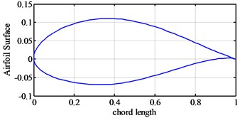
NACA63418 wind turbine blade airfoil is selected as the research object, whose shape is shown in Fig. 1. The physical parameters of primary air are used in the simulation as follows:

Air velocity ( $V_{0}$ ) is 12 m/s, atmospheric pressure ( $P$ ) is 101325 Pa, air density ( $ρ$ ) is 1.225 kg/m, air temperature ( $T$ ) is 288 K, kinematic viscosity) ( $v$ ) is 1.46110×10^-5 m²/s.

Fig. 1NACA63418 airfoil shape

The theoretical aerodynamic performance values of NACA63418 airfoil can be obtained from the PROFILI program. When the angle of attack is at 8°, the lift-drag coefficient gets maximal, that is, the best angle of attack is 8°. The maximal lift coefficient is 1.121 and the maximal drag coefficient is 0.02686.

4. Airfoil grid meshing

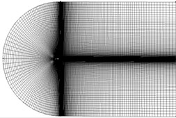
The simulation of the blade airfoil begins with the airfoil calculating field firstly. The appropriate selection of the calculation of the flow area has an important influence on the simulation results. In principle, the boundary is as far as possible [10], but it also increases the amount of computation and the result may not be the best. According to the experiences of predecessors [11] the selected airfoil field range is 10 times of the chord length, the grid shape is C-shape which can make the mesh generation convenient.

The unstructured meshing method is used to mesh the airfoil grid [12]. Fig. 2 shows the integral mesh grid of the flow field of wind turbine blade airfoil.

Fig. 2The integral mesh grid

5. Simulation and results

5.1. Simulation conditions

In order to investigate the impacts of different turbulence models on the wind turbine blade airfoil, the introduced three kinds of turbulence models are applied to numerically simulate under the same Reynolds number of 2.5×10⁶, and the same air velocity of 12 m/s. The characteristic length of the NACA63418 airfoil is 1 m. SIMPLE algorithm is used in processing coupling problems of speed and pressure in FLUENT solver. The second-order upwind scheme is used to discrete. And the residual magnitude is controlled as 10^-6.

The angle of attack is determined within 0° and 16°, and the lift coefficient and drag coefficient of the NACA63418 airfoil are aerodynamically calculated and simulated every 2° of angle of attack.

5.2. Simulation and comparison of the lift coefficient

The theoretical values of the lift coefficients of selected airfoil are compared with the simulated lift coefficients of three turbulence models respectively. Fig. 3 shows the comparison of the lift coefficients simulated by three turbulent models and the theoretical lift coefficient. In order to verify the simulation results of lift coefficients of three turbulent models, the flow fields given by three turbulent models are also given subsequently as Figs. 4-6.

According to Fig. 3, the simulated lift coefficients of the theoretical value and three different turbulence models are very close during the attack angle of 0°-8° range and more consistent with the theoretical values. Lift coefficient increases nearly linearly with the increasing attack angle when the attack angle is smaller than 8°. The lift coefficient results of three turbulence models show significant differences when the angle of attack is bigger than 8°. The stall point forecasts of the different turbulent models are also different.

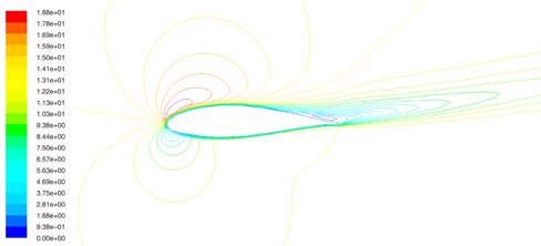
From Fig. 4, three different turbulent models were also applied to simulate the fluid field respectively. When the angle of attack is 8°, the flow field of the trailing edge of wind turbine blade airfoil shows that the flow still belongs to laminar status for three turbulent models, and there are no turbulence and flow separation at all. That is why the simulation results of aerodynamic performance of blade airfoil using three turbulent models are very near when the angle of attack is below 8° and coincide with the theoretical value very much.

Fig. 3The comparison of lift coefficient using different model

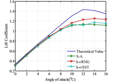
Fig. 4The flow fields of wind turbine blade airfoil when angle of attack is 8°

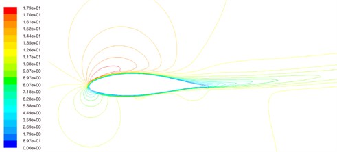
a) S-A model

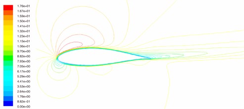
b) k-εRNG model

c) k-ωSST model

According to Fig. 3, the lift coefficient simulated by S-A model reaches maximal point when the attack angle is 12° and the theoretical value of the lift coefficient is also maximal when the attack angle is 12°, then airfoil enters the stall area with the increasing attack angle and the lift coefficient sudden declines. Therefore the S-A model predicts more accurate as for the stall point than the other two turbulent models.

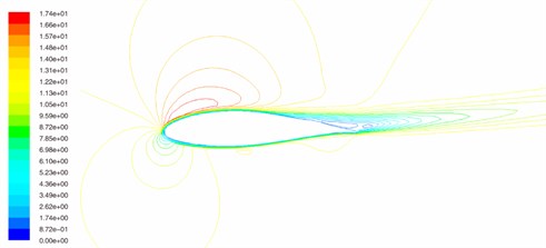
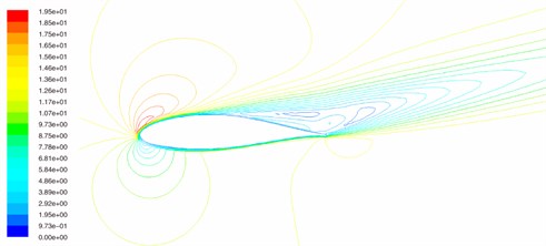
Fig. 5The flow fields of wind turbine blade airfoil when angle of attack is 12°

a) S-A model

b) k-εRNG model

c) k-ωSST model

From Fig. 5, when the angle of attack is 12°, for S-A turbulent model as Fig. 5(a), the flow field of trailing edge of wind turbine blade airfoil begins to separate, so the airfoil begins to enter the stall area, and lift coefficient begins to decease. And that is why the lift coefficient given by the S-A turbulent model reaches maximal. For k-εRN model as Fig. 5(b) and k-ωSST model as Fig. 5(c), the flow field of trailing edge of wind turbine blade separates. When the angle of attack is bigger than 12°, the blade airfoil doesn’t enter the stall area, so the lift coefficient goes on increasing.

According to Fig. 3, The lift coefficient calculated by k-εRNG model increases linearly with the increasing attack angle and reaches maximal when the attack angle is 14°, then enters into the stall area, the forecast for the stall point is relatively late, but the lift coefficient simulated by k-εRNG is more closer to the theoretical value after it enters the stall area. The k-εRNG simulated curve is also more consistent with the theoretical curve on the changing trend of the curve, and the iterative times are between S-A model and k-ωSST model.

The lift coefficient simulated by k-ωSST model is worse than the result from k-ωSST model when the airfoil enters into the stall area. The lift curve decrease relatively flat and has large differences with the theoretical curve, the forecast for the stall point is also relatively late and not very obviously.

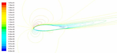
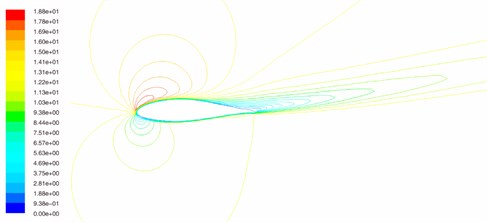
Fig. 6The flow fields of wind turbine blade airfoil when angle of attack is 14°

a) S-A model

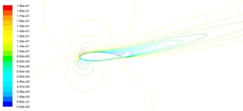
b) k-εRNG model

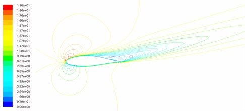
c) k-ωSST model

From Fig. 6, when the angle of attack is 14°, for S-A turbulent model as Fig. 6(a), the flow field of trailing edge of wind turbine blade airfoil separates very violently, the airfoil enters the stall area deeply, and lift coefficient deceases very dramatically. This also coincides with the Fig. 3. The flow field given by k-εRN model as Fig. 6(b) and k-ωSST model as Fig. 6(c) begin to enter stall area, the flow field of trailing edge of wind turbine blade separates slightly. Therefore, the lift coefficients of given by k-εRN model and k-ωSST model reaches maximal when the angle of attack is 14°.

We can conclude that the lift coefficients of three turbulent models are correct based on the simulation of flow field of wind turbine blade airfoil. Then the drag coefficient and ratios of lift coefficient to drag coefficient are researched in the following part.

5.3. Simulation and comparison of the drag coefficient

Under the same conditions with the lift coefficient, Fig. 7 shows the comparison of the drag coefficient simulated by three turbulent models and the theoretical lift coefficient.

From Fig. 7, the drag coefficient curve of the four conditions, the drag coefficient simulated by S-A model complies with the theoretical value before the best angle of attack.

The drag coefficient and the deviation simulated by S-A, k-εRNG and k-ωSST turbulence models are sequentially increased with the theoretical value and the iterative times also increase in turn. After the best angle of attack, the drag coefficient simulated by k-εRNG model is very consistent with the theoretical value.

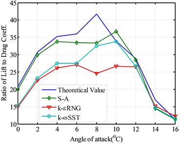
5.4. Ratios of lift coefficient to drag coefficient

In order to investigate the aerodynamic simulation of the ratio of lift coefficient to drag coefficient, Fig. 8 shows the ratios of lift coefficient to drag coefficient for the theoretical value and three turbulent models. The best angle of attack decided by the theoretical value is 8°. However, three kinds of turbulence models can not provide good numerical simulation of the best angle of attack of the wind turbine blade airfoil. These three turbulence models forecast the best angle of attack as 10° at the same time. Therefore, as for the forecasts of the best angle of attack, three turbulence models can’t provide the good simulation results.

Fig. 7The comparison of drag coefficient using different models

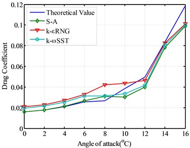
Fig. 8The comparison of ratios of lift coefficient to drag coefficient

5.5. Aerodynamic simulation with combined turbulent model

Comparing the simulated lift and drag coefficient with the theoretical value, the S-A turbulence model is not only more accurate before the best attack angle but also has a best forecast for the airfoil stall point. However, after the best attack angle, the k-εRNG turbulence model is much more appropriate for the simulation of the aerodynamic performance of the wind turbine blade airfoil. In the past literature, there is only one turbulence model can be used to simulate the aerodynamic performance. Therefore, during different range of the angle of attack, the different turbulent model should be applied for the simulation of aerodynamics of the blade airfoil, respectively, which can benefit to the aerodynamic design and analysis of the wind turbine blade airfoil.

Considering the lift coefficient and drag coefficient of each model, the ratio of lift coefficient to drag coefficient, a combined turbulence model, that is, applying S-A before the best angle of attack and k-εRNG model after best angle of attack, was put forward to simulate the aerodynamic performance of wind turbine blade airfoil.

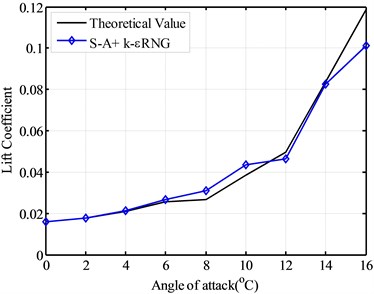
Fig. 9 gives the simulated lift coefficient given by combined turbulence model, S-A and k εRNG. Fig. 10 shows simulated the drag coefficient given by combined turbulence model, S-A and k-εRNG.

From Fig. 9 and Fig. 10, the lift coefficient and drag coefficient of the combined turbulence model of the selected airfoil model, show the better results than the simulation results of one turbulence model, when only one of the S-A model, k-εRNG model and k-ωSST turbulence model was used. Although there are still relative large error for the stall point and the best angle of attack between the theoretical values and the combined turbulence model, the combined turbulence model provides the better simulation results for the lift coefficient and drag coefficient. If there are other turbulence model which be applied to simulate the aerodynamic performance of wind turbine blade airfoil, a new combined model can also be put forward. The so-called combined turbulence model can be used for the further and better simulation results of aerodynamic performance in the future.

Fig. 9The lift coefficient using combined model

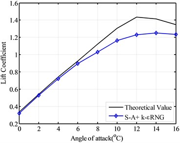
Fig. 10The drag coefficient using combined model

6. Conclusions

NACA63418 wind turbine blade airfoil was selected as the research subject, the S-A, k-εRNG and k-ωSST turbulence models were applied to simulate the selected airfoil respectively, in order to obtain the aerodynamic performance of wind turbine blade airfoil. When the simulated aerodynamic performances were compared with the theoretical value of the airfoil, it can be found one single turbulence model can’t provide the good simulation results according to the size of the errors, the forecast of the stall point, the iterative time and the best angle of attack. Based on the traditional one single turbulence model for aerodynamic performance, a brand-new combined turbulence model, using the S-A turbulence model before the best attack angle and using the k-εRNG turbulence model after the best attack angle is more appropriate for the simulation of the aerodynamic performance, for the combined model can give the better simulation results for the dominant aerodynamic performance, lift coefficient and drag coefficient. The simulation approach of combined turbulence model can overcome the effects of a single numerical simulation result of the aerodynamic performance of the airfoil.

References

Hansen M. O. L. Aerodynamics of Wind Turbines. James & James, London, 2008.

Search CrossRef
Lee D. Application of computational fluid dynamics in transonic aerodynamic design. American Institute of Aeronautics and Astronautics, Aerospace Sciences Meeting and Exhibition, 1993.

Search CrossRef
Madsen H., Sorensen N., Schreck S. Yaw aerodynamics analyzed with three codes in comparison with experiment. Wind Energy Symposium, Reno, USA, 2003, p. 94-103.

Search CrossRef
Lubitz W. D. Impact of ambient turbulence on performance of a small wind turbine. Renewable Energy, Vol. 61, 2014, p. 69-73.

Search CrossRef
Sunderland K., Woolmington T., Blackledge J., Conlon M. Small wind turbines in turbulent (urban) environments: a consideration of normal and Weibull distributions for power prediction. Journal of Wind Engineering and Industrial Aerodynamics, Vol. 121, 2013, p. 70-81.

Search CrossRef
Walter P. W., Stuart S. O. CFD calculations of s809 aerodynamic characteristics. American Institute of Aeronautics and Astronautics, Aerospace Sciences Meeting and Exhibition, 1997, p. 1-8.

Search CrossRef
Duque E. P. N., Burklund M. D., Johnson W. Navier-stokes comprehensive analysis performance predictions of the NREL phase VI experiment. Journal of Solar Energy Engineering, Vol. 125, 2003, p. 457-467.

Search CrossRef
Elkhoury M. Assessment and modification of one-equation models of turbulence for wall bounded flows. Journal of Fluids Engineering, Vol. 129, 2007, p. 921-928.

Search CrossRef
Rahman M. M. Evaluating k-ε with one-equation turbulence model. Procedia Engineering, Vol. 56, 2013, p. 206-216.

Search CrossRef
Hand M. M., Simms D. A. Unsteady aerodynamics experiment phase VI: wind tunnel test configurations and available data campaigns. National Renewable Energy Laboratory, Technical reportr, NREL/ TP 2500-29955, 2001.

Search CrossRef
Schepers J. G., Feigl L., Rooij R. V., Bruining A. Analysis of detailed aerodynamic field measurements using results from an aeroelastic code. Wind Energy, Vol. 7, Issue 4, 2004, p. 357-372.

Search CrossRef
Lindenburg C. Investigation into rotor blade aerodynamics. Report Number ECN-C-03-025, 2003.

Search CrossRef

About this article

Received

26 December 2013

Accepted

20 July 2014

Published

15 August 2014

Keywords

turbulence models

wind turbine

blade airfoil

aerodynamic performance

numerical simulation

Acknowledgements

The work was supported by the Shanghai Natural Science Foundation under Grant No. 11ZR1414200.

This is an open access article distributed under the Creative Commons Attribution License, which permits unrestricted use, distribution, and reproduction in any medium, provided the original work is properly cited.