Direct solution of Navier-Stokes equations by using an upwind local RBF-DQ method

Sun, Dan; Ai, Yanting; Zhang, Wanfu; Yang, Jiangang

Journal of Vibroengineering

Browse Journal

Submit article

Published: 15 February 2014

Check for updates

Direct solution of Navier-Stokes equations by using an upwind local RBF-DQ method

Dan Sun¹

Yanting Ai²

Wanfu Zhang³

Jiangang Yang⁴

^{1, 2}Liaoning Key Lab of Advanced Test Technology for Aerospace Propulsion System Shenyang Aerospace University, Shenyang 110136, China

^{3, 4}National Engineering Research Center of Turbo-Generator Vibration Southeast University, Nanjing 210096, China

Corresponding Author:

Wanfu Zhang

Cite the article Download PDF

Downloads 1255

WoS Core Citations 5

Abstract

The differential quadrature (DQ) method is able to obtain quite accurate numerical solutions of differential equations with few grid points and less computational effort. However, the traditional DQ method is convenient only for regular regions and lacks upwind mechanism to characterize the convection of the fluid flow. In this paper, an upwind local radial basis function-based DQ (RBF-DQ) method is applied to solve the Navier-Stokes equations, instead of using an iterative algorithm for the primitive variables. The non-linear collocated equations are solved using the Levenberg-Marquardt method. The irregular regions of 2D channel flow with different obstructions situations are considered. Finally, the approach is validated by comparing the results with those obtained using the well-validated Fluent commercial package.

1. Introduction

Many computational methods have been applied to solve the Navier-Stokes equation, prominent among which are the finite differential method (FDM), the finite element method (FEM) and the finite volume method (FVM). Although these methods have been successfully applied to many engineering situations, their accuracy highly depends on mesh quality. Specifically, appropriate mesh generation is typically a major challenge in computational fluid dynamics (CFD). Moreover, the mesh generation, modification and re-meshing become difficult and time-consuming when the geometry of the problem is complex. Thus, numerical simulations and solution procedures using these traditional methods are often limited by slow mesh generation.

In the past decade, the so-called mesh-free methods have became one of the attractive research areas in computational mechanics. A number of meshless methods have been proposed to date. These methods include the smoothed particle hydrodynamics method (SPH) [1], the diffuse element method (DEM) [2], the element-free Galerkin method (EFGM) [3], the reproducing kernel particle method (RKPM) [4], the partition of unity method (PUM) [5], the hp-clouds method (HPCM) [6], the finite point method (FPM) [7], the meshless local Petrov-Galerkin method (MLPGM) [8], the moving-particle semi-implicit method (MPSM) [9] and the general finite difference method (GFDM) [10]. Recently, a new meshless method was proposed based on the so-called radial basis functions (RBFs), have become attractive for solving Partial differential equations (PDEs). Initially, RBFs were developed for multivariate data and function interpolation, especially for higher dimension problems. However, their “truly” mesh-free nature motivated researchers to use them to deal with PDEs. Kansa [11, 12] initiated the concept of solving PDEs by using RBFs. Since the resultant coefficient matrix of Kansa’s method is not symmetric, Fasshauer [13] proposed the Hermite type method, which can generate symmetric coefficient matrix that guarantees the related linear equations being solvable. Other great contributions to solve PDEs by using RBFs include the work presented by Demirkaya [14], Fornberg [15], Hon and Wu [16], Chen and Tanaka [17], Chen [18], Xiang [19] et al. The advantages of RBFs-based methods have been summarized by Wu [20] as follows: (1) it is a truly mesh-free algorithm; (2) it is space dimension independent in the sense that the convergence order is of $O (h d + 1)$ where $h$ is the density of the collocation points and $d$ is the spatial dimension.

Unfortunately, the numerical schemes based on RBFs to solve PDEs proposed up to date have one feature in common, i.e., they are actually based on the function approximation. In other words, these methods directly substitute the expression of function approximation by RBFs into a PDE, and then change the dependent variables into the coefficients of function approximation. The process is very complicated, especially for nonlinear problems. Thus, the method has not been extensively applied to solve practical problems. The objective of this paper is to present a numerical scheme, which is simple to be implemented for linear and nonlinear problems. The method preserves the properties of high accuracy and mesh freeness of RBFs and the derivative approximation directly through the differential quadrature (DQ) methodology [21]. The DQ technique originates from the integral quadrature. The basic idea of the DQ method is that the derivatives of unknown function can be approximated in terms of the function values at a set of points, either uniformly or randomly distributed. Numerical experiments showed that the combination of DQ technique and RBFs provides a novel and effective algorithm for the use of RBFs to solve PDEs.

Furthermore, as observed by Shu et al. [22] and Sun et al. [23], the DQ method is limited in application to regular regions by its quadrature rules, such as rectangular and parallelogram regions, or circular, concentric, and sectorial regions. When an irregular region must be considered, the implementation of the DQ method becomes difficult. In addition, the upwind mechanism is necessary in numerical computation of fluid flow, but the DQ method lacks the upwind mechanism to characterize the convection of the fluid flow.

To overcome the difficulties and drawbacks mentioned above, a local RBF-based differential quadrature method (RBF-DQ) is developed in this paper. It can handle irregular regions conveniently and possesses the upwind mechanism. Specifically, compared with the classical iterative approach, a local RBF-DQ method is proposed to directly approximate the derivatives, in which RBFs are formed by using local supporting knots. This method is very flexible as it does not requires extra effort on the division of the computational domain. We collocate the fully non-linear Navier-Stokes equations and solve the resulting non-linear system directly using the Levenberg-Marquardt method. The approach present a novel approach for accurate and stable solution of the Navier-Stokes equations using upwind local RBF-DQ method. It seems to produce accurate and stable results compared to the conventional iterative methods. The proposed numerical scheme is applied to determine the velocity and pressure for the flow through a channel with the obstructions in different patterns. The predicted channel flow results mirror the analytical solutions, while the 2D results compare favorably with those obtained using the well-validated CFD-Fluent commercial package.

2. Numerical methodology

2.1. Systems

Three types of geometry are considered as shown in Fig. 1. Fig. 1a shows a 2D flow between two flat plates with one rectangular obstacle placed at the center of the bottom plate, Fig. 1b shows a 2D flow between two flat plates with two rectangular obstacles, Fig. 1c shows a 2D flow between two flat plates with three rectangular obstacles in staggered pattern. The above models all belong to irregular step flow, which is classical CFD model.

The meshless method requires a complete set of boundary conditions in order to obtain a solution. In this study, the no-slip condition is imposed on all walls, implying zero velocity on the walls for the 2D channel flow. The inflow velocity for the 2D channel flow is specified by a mean velocity $U_{\infty}$ . The $x$ -component of velocity is assumed to be equal to $U_{\infty}$ at the inlet, the $y$ -component of velocity is assumed to be zero, and the pressure is a reference gage value of zero. The outlet is located sufficiently far from the inlet ( $L = 10 H$ ) to ensure fully-developed flow in the channel. At the outlet, we assume that the flow exits with straight streamlines, the gradients of all variables are zero in the flow direction and the continuity equation is satisfied. The wall and outlet pressure boundary equations are obtained by taking the scalar product of the momentum equation with the outward normal to the boundary. These boundary conditions are summarized in Table 1.

Fig. 1Different models of the system used for computational experiments

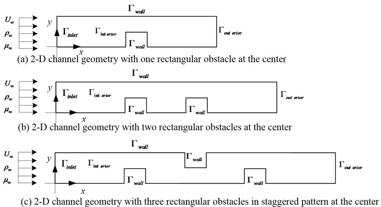
Table 1Boundary conditions

	Velocity	pressure
$Γ_{w a l l}$	$u^{} = 0, v^{} = 0$	$- \frac{\partial p^{}}{\partial y^{}} + \frac{1}{R e} (\frac{\partial^{2} v^{}}{\partial x^{ 2}} + \frac{\partial^{2} v^{}}{\partial y^{ 2}}) = 0, (f o r n y \neq 0 a n d n x = 0)$ $- \frac{\partial p^{}}{\partial y^{}} + \frac{1}{R e} (\frac{\partial^{2} u^{}}{\partial x^{ 2}} + \frac{\partial^{2} u^{}}{\partial y^{ 2}}) = 0, (f o r n x \neq 0 a n d n y = 0)$
$Γ_{i n l e t}$	$u^{} = 1, v^{} = 0$	$p^{*} = 0$
$Γ_{o u t l e t}$	$\frac{\partial u^{}}{\partial x} = 0, \frac{\partial v^{}}{\partial x} = 0$	$\frac{\partial p^{*}}{\partial x} = 0$

2.2. Governing equation

In this section, the local RBF-DQ method with upwind mechanism is described. It is then used to predict the velocity and pressure distribution in a two-dimensional channel flow. The flow is assumed to be steady, viscous and incompressible. The Navier-Stokes equations for the flow in Cartesian coordinates are:

1

\{\begin{array}{l} \frac{\partial u^{*}}{\partial x^{*}} + \frac{\partial v^{*}}{\partial y^{*}} = 0, \\ u^{*} \frac{\partial u^{*}}{\partial x^{*}} + v^{*} \frac{\partial u^{*}}{\partial y^{*}} = - \frac{\partial p^{*}}{\partial x^{*}} + \frac{1}{R e} (\frac{\partial^{2} u^{*}}{\partial {x^{*}}^{2}} + \frac{\partial^{2} u^{*}}{\partial {y^{*}}^{2}}), \\ u^{*} \frac{\partial v^{*}}{\partial x^{*}} + v^{*} \frac{\partial v^{*}}{\partial y^{*}} = - \frac{\partial p^{*}}{\partial y^{*}} + \frac{1}{R e} (\frac{\partial^{2} v^{*}}{\partial {x^{*}}^{2}} + \frac{\partial^{2} v^{*}}{\partial {y^{*}}^{2}}), \end{array}

where all variables are non-dimensional, $u^{*}$ and $v^{*}$ represent the velocity components in the Cartesian coordinate directions $x^{*}$ and $y^{*}$ , respectively. $p^{*}$ is the pressure, $R e$ is the Reynolds number ( $ρ U_{\infty} D / μ_{\infty}$ ) where $D$ is the characteristic length of the domain. $ρ_{\infty}$ and $U_{\infty}$ are the reference density and mean velocity, respectively. The Cartesian coordinates x* and y* are non-dimensional with respect to $D$ , $u^{*}$ and $v^{*}$ are non-dimensional with respect to $U_{\infty}$ , $p^{*}$ is non-dimensional with respect to the dynamic pressure $ρ U_{\infty}^{2}$ .

2.3. Upwind local RBF-DQ method

The DQ method is a numerical discretization technique for approximation of derivatives. The essence of the DQ method is that the partial derivative of an unknown function with respect to an independent variable is approximated by a weighted linear sum of function values at all discrete points. Suppose that a function $f (x)$ is sufficiently smooth. Then its $m$ -th order derivative with respect to $x$ at a point $x_{i}$ can be approximated by DQ as:

2

{\frac{\partial^{m} f}{\partial x^{m}} |}_{x = x_{i}} = \sum_{j = 1}^{N} w_{i, j}^{(m)} f (x_{j}), i = 1,2, \dots, N,

where $x_{j}$ are the discrete points in the domain, $f (x_{j})$ and $w_{i j}^{(m)}$ are the function values at these points and the related weighting coefficients. Obviously, the key procedure in the DQ method is the determination of the weighting coefficients $w_{i, j}^{(m)}$ .

Due to excellent performance of RBFs in the function approximation, they are chosen as the base functions to determine the weighting coefficients $w_{i, j}^{(m)}$ in this work. There are many RBFs (expression of $φ$ ) available. The most commonly used RBFs are:

(a) Multi-quadratics (MQs): $φ (r) = \sqrt{r^{2} + c^{2}}$ , $c > 0$ ;

(b) Thin-plate splines (TPS): $φ (r) = r^{2 n} l o g (r)$ , $n$ is an integer;

(c) Gaussians: $φ (r) = e^{- c r^{2}}$ , $c > 0$ ;

(d) Inverse MQs: $φ (r) = \frac{1}{\sqrt{r^{2} + c^{2}}}$ , $c > 0$ ,

where $r = ‖ x - x_{k} ‖$ represents the Euclidean norm, and $c$ is a free shape parameter. The shape parameter $c$ defined in the MQs and Gaussian basis functions has an important role in the approximation of the meshless methods. Although analysis are available for the shape parameter [24], there is no mathematical theory on choosing its optimal value. In the following section, we will to determine the value by using use TPS RBF which does not require a shape parameter and its solution is not dependent on this parameter. Navier–Stokes equations are of second order, and we want to improve and extend this method to 3D problems, so we must use a higher order TPS [25, 26] and the integer $n$ will be chosen as 2.

Substituting the set of TPS RBF into Eq. (2), the determination of corresponding coefficients for the first-order derivative is equivalent to solving the following linear equations:

3

\frac{\partial φ (X_{I})}{\partial x} = \sum_{j = 0}^{N_{I}} w_{I, j}^{(1 x)} φ_{k} (X_{I}^{j}), k = 0,1, 2, \dots, N_{I},

(for simplicity, the notation $φ_{k} (X)$ is adopted to replace $φ (‖ x - x_{k} ‖)$ ) or in the matrix form:

4

\underset{\{\frac{\partial φ (X_{I})}{\partial x}\}}{\underset{⏟}{[\begin{matrix} \frac{\partial φ_{0} (X_{I})}{\partial x} \\ \frac{\partial φ_{2} (X_{I})}{\partial x} \\ ⋮ \\ \frac{\partial φ_{N_{I}} (X_{I})}{\partial x} \end{matrix}]}} = \underset{[A]}{\underset{⏟}{[\begin{matrix} φ_{0} (X_{I}^{0}) & φ_{0} (X_{I}^{1}) & \dots & φ_{0} (X_{I}^{N_{I}}) \\ φ_{1} (X_{I}^{0}) & φ_{1} (X_{I}^{1}) & \dots & φ_{1} (X_{I}^{N_{I}}) \\ ⋮ & ⋮ & ⋱ & ⋮ \\ φ_{N_{I}} (X_{I}^{0}) & φ_{N_{I}} (X_{I}^{1}) & \dots & φ_{N_{I}} (X_{I}^{N_{I}}) \end{matrix}]}} \underset{\{w\}}{\underset{⏟}{[\begin{matrix} w_{I, 0}^{(1 x)} \\ w_{I, 1}^{(1 x)} \\ ⋮ \\ w_{I, N_{I}}^{(1 x)} \end{matrix}]}} .

Therefore, if the collocation matrix $[A]$ is non-singular, the coefficient vector [19] can be obtained by:

5

\{w\} = {[A]}^{- 1} \{\frac{\partial φ (X_{I})}{\partial x}\} .

The non-singularity of the collocation matrix $[A]$ depends on the properties of RBFs used. According to the work of [25], the matrix $[A]$ is conditionally positive definite for TPS RBFs. This fact guarantees the nonsingularity of matrix $[A]$ for distinct supporting points. The coefficient vector ${w}$ can be used to approximate the first-order derivative in the $x$ -direction for any locally smooth function at node $x_{I}$ . The calculation of weighting coefficients for other derivatives can follow the same procedure.

It is clear that the implementation of the DQ method becomes difficult when an irregular region must be considered. The essential reason behind this is the method lacks the upwind mechanism. Therefore, DQ method using to calculate the flow field characteristics with high Reynolds number will bring error. To overcome the difficulties and drawbacks, a local RBF-DQ method with upwind mechanism is utilized in this paper. Unlike the RBF-DQ method, derivative of a function with respect to a coordinate direction at an internal grid point is expressed as a weighted liner sum of the function values at partial grid points along that coordinate direction rather than at all grid points.

Fig. 2The local support domain model with upwind scheme (al=3, ar=2)

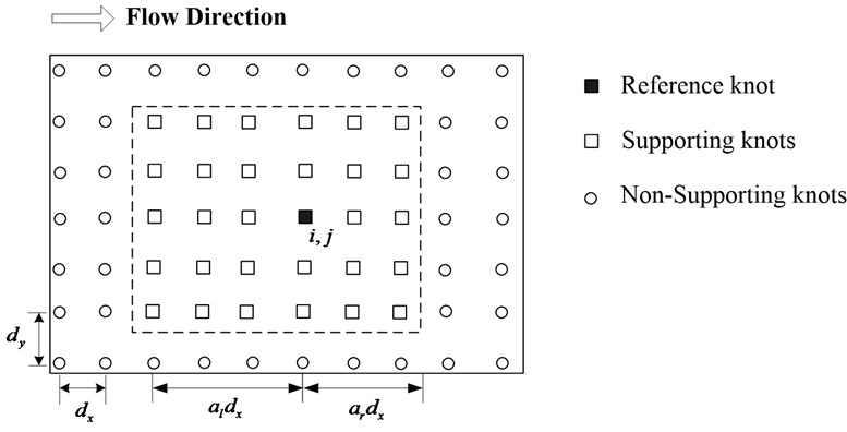
Local RBF-DQ method uses local support domain point function to approximate the partial derivatives of a function:

6

{\frac{\partial^{m} f}{\partial x^{m}} |}_{x = x_{i}} = \sum_{j = 1}^{n} w_{i, j}^{(m)} f (x_{j}),

$n$ is the number of the local support domain points.

7

x_{i} - a_{l} d_{x} \leq x_{j} \leq x_{i} + a_{r} d_{x},

$a_{l}$ and $a_{r}$ are the upstream and downstream support domain coefficients. $a_{l} > a_{r}$ , $d_{x}$ is the mean interval in the $x$ direction.

The local support domain model with upwind scheme is considered as shown in Fig. 2.

2.4. Expansion of the Navier-Stokes by upwind local RBF-DQ method

By using the upwind RBF-DQ method described above, Eq. (1) can be discretized as the following formula:

8

\{\begin{array}{l} \sum_{k = 1}^{n} w_{i, k}^{1 x} u_{i} + \sum_{k = 1}^{m} w_{i, k}^{1 y} v_{i} = 0, \\ u_{i} \sum_{k = 1}^{n} w_{i, k}^{1 x} u_{i} + v_{i} \sum_{k = 1}^{m} w_{i, k}^{1 y} u_{i} + \sum_{k = 1}^{n} w_{i, k}^{^{1 x}} p_{i} - \frac{1}{R e} [\sum_{k = 1}^{n} w_{i, k}^{2 x} u_{i} + \sum_{k = 1}^{m} w_{i, k}^{2 y} u_{i}] = 0, \\ u_{i} \sum_{k = 1}^{n} w_{i, k}^{1 x} v_{i} + v_{i} \sum_{l = 1}^{m} w_{i, k}^{1 y} v_{i} + \sum_{k = 1}^{n} w_{i, k}^{^{1 y}} p_{i} - \frac{1}{R e} [\sum_{k = 1}^{n} w_{i, k}^{2 x} v_{i} + \sum_{k = 1}^{m} w_{i, k}^{2 y} v_{i}] = 0 . \end{array}

The traditional pressure-correction methods are widely used to solve N-S equations. An example of this approach is the SIMPLE algorithm [27]. This method integrates the Navier-Stokes equations in time at each time-step by firstly solving the momentum equations using an approximate pressure field to yield an intermediate velocity field that will not, in general, satisfy continuity. A Poisson equation is then solved with the divergence of the intermediate velocity as a source term to provide a pressure correction, which is then used to correct the intermediate velocity field, providing a divergence free velocity. The pressure is updated and integration then proceeds to examine the convergence. If the solution is converged the results are finalized. If not, the iterative process continues from the momentum equation with the new pressure and velocity field.

Kassab and Divo [28] combined the pressure-correction method with the radial basis collocation method to solve heat diffusion–advection problems. Their approach, which is similar to the SIMPLE algorithm, is summarized as follows: The solution algorithm starts with an initial velocity field, which satisfies continuity, then the velocity field is introduced in the N-S equations, and the time derivatives are approximated using backward differencing, transforming the N-S to the Helmholtz Poisson equation set for estimating the velocity field. Once the Helmholtz Poisson problem is solved, the velocity field is updated and forced to satisfy continuity. An equation to update the pressure field is obtained by taking the divergence of the momentum equation and applying the continuity equation. The Poisson equation for the pressure field can be solved by imposing a proper and complete set of boundary conditions.

Our approach is distinct from above, instead, we use a least-square method, which is inherently iterative, to find primitive variables ( $u$ , $v$ and $p$ ) directly. The N-S and the boundary condition equations together constitute a system of non-linear equations, which are to be solved. These non-linear equations are then solved by one of the least-square methods, Levenberg-Marquardt. At the end we obtain the solutions of the velocity and pressure field directly. This procedure is described in detail below.

The Navier-Stokes and boundary condition equations together constitute a set of non-linear equations, which are to be solved. The expanded velocity and pressure terms and their first and second derivatives are directly inserted into the equations. The boundary condition equations are collocated at the boundary points $(i = 1, \dots, N B)$ and the continuity and momentum equations are collocated at the interior domain points $(i = N B + 1, \dots, N B + N I)$ . Then a non-linear system of equations can be solved by the least-square optimization techniques such as the Levenberg-Marquardt method [29]. The Levenberg-Marquardt algorithm is an iterative technique that locates the minimum of a multivariate function that is expressed as the sum of squares of non-linear real-valued functions. It has became a standard technique for non-linear least-squares problems. The reader is referred to the literature [29] for further details of this method.

3. Numerical results and discussions

Our objective in the paper is to demonstrate the feasibility of the direct solution approach using the upwind local RBF-DQ method. Once the feasibility established in both 2D and 3D cases, we will set about optimization of the technique and code. The parameters are chosen as $R e = 100$ , $200$ and $300$ , the three cases were chosen after systematic analysis of a number of examples over a wide range of $R e$ . The 2D channel flow predictions are compared with those obtained using the finite volume method (FVM) which is embodied in the CFD-Fluent computational package. In order to perform error analysis, the relative percent error ( $ε$ ) is calculated for each node, and then the arithmetic mean ( $μ$ ) and the standard deviation ( $σ$ ) of the relative error are calculated for each case, using the following expressions:

9

ε = 100 \times (\frac{X_{R B F - D Q} - X_{C F D - F l u e n t}}{X_{C F D - F l u e n t}}),

10

μ = \frac{1}{N} \sum_{i = 1}^{N} ε_{i},

11

σ = \sqrt{\frac{1}{N} \sum_{i = 1}^{N} {(ε_{i} - μ)}^{2}},

in which $X$ is any generic variable (velocity, pressure, stream function).

3.1. Gird-independence study

In the present study, a number of different grid sizes are considered in order to check the sufficiency of the mesh resolution. Table 2 depicts the comparisons of error and CPU times between RBF-DQ method and CFD-Fluent method in the different mesh density, three different mesh sizes are used for discretization in the three flow types. It can be clearly seen that the error $μ$ and $σ$ decrease as the node density increases.The upwind codes have a tendency to loose stability at higher distance between nodes.

As expected, the CPU time for the meshless method depends on the number of nodes employed, as well as the Levenberg-Marquardt convergence criteria. However, a comparison of the results (following section) indicates that the node numbers in Table 2 provide sufficiently accurate results. Considering that there is still some improvement for optimization of the RBF code in the future, the computational cost as indicated in Table could be considered comparable to the commercial codes.

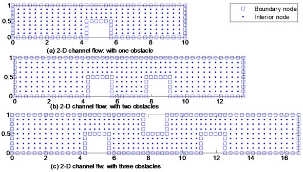
Consider the error and CPU time, the distribution of nodes in the domain for the flow situations considered is shown in Fig. 3. Fig. 3a depicts 2D channels with one obstacle on the lower wall, Fig. 3b represents 2D channels with two obstacles on the lower wall and Fig. 3c involves flow through a 2D channel with three obstructions in staggered pattern. The obstruction is located mid-way between the inlet and the outlet. The non-dimensional length of the obstruction is 1.4, and the height is 0.5 in all cases. Fig. 3 shows that for 2D channels flow with one obstacle, a total of 86 collocation points are used on the boundary and 186 collocation points are used in the interior for RBF-DQ expansion. For channel flow with two obstructions, we used a total of 118 collocation points on the boundary and 246 collocation points in the interior. A total of 150 collocation points are used on the boundary and 306 collocation points in the interior channel with three obstructions.

Table 2The comparisons of error and CPU times between RBF-DQ method and CFD-Fluent method in the different mesh density (Re=100)

Flow type	Boundary nodes	Interior nodes	Total nodes	CPU time (s)	CFD-Fluent (s)	Error
Flow type	Boundary nodes	Interior nodes	Total nodes	CPU time (s)	CFD-Fluent (s)	$μ$ (%)	$σ$ (%)
Channel flow with one obstruction	43	93	136	380	260	8.90	12.6
	86	186	272	405	280	1.61	3.25
	172	372	544	456	405	1.24	2.51
Channel flow with two obstructions	59	123	184	412	275	9.65	15.61
	118	246	364	435	310	3.57	4.23
	236	492	728	512	396	3.18	3.96
Channel flow with three obstructions	75	153	228	434	328	10.51	18.44
	150	306	456	510	350	4.78	5.06
	300	612	912	582	471	4.25	4.81

Fig. 3Node distribution for 2-D channel flow considered

3.2. Influence of upwind support domain on the numerical results

The upwind mechanism is important to the numerical computation of fluid flow. Table 3 shows the comparison of error in the different upwind support domain coefficients, it is shown that the upwind support domain can improve the accuracy of the numerical result. As $R e$ increases, the upstream support domain coefficient is bigger than the downstream support domain coefficient.

Table 3The comparison of error in the different upwind support domain coefficients (channel flow with one obstruction)

Support domain coefficients	$R e = 100$		$R e = 200$		$R e = 300$
Support domain coefficients	$μ$ (%)	$σ$ (%)	$μ$ (%)	$σ$ (%)	$μ$ (%)	$σ$ (%)
$a_{l} = 2$ , $a_{r} = 2$	4.56	6.98	6.28	7.94	7.27	9.25
$a_{l} = 3$ , $a_{r} = 2$	1.61	3.25	2.38	3.77	3.45	4.89
$a_{l} = 4$ , $a_{r} = 2$	4.28	6.54	4.83	5.22	3.10	4.34

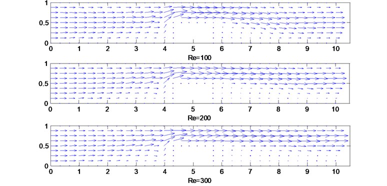
Fig. 4Predicted velocity vector for 2D channel flow

(a) 2D channel flow with one obstruction

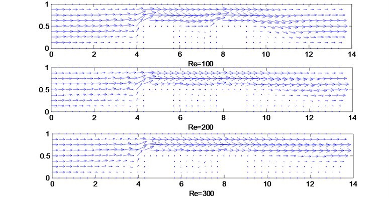
(b) 2D channel flow with two obstructions

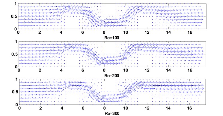
(c) 2D channel flow with three obstructions

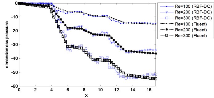
Fig. 5Predicted pressure distribution along the lower wall for 2D channel flow

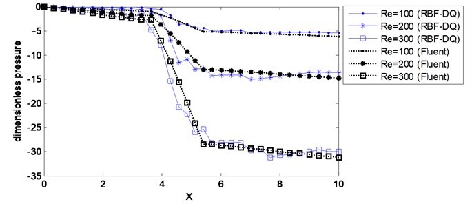
(a) 2D channel flow with one obstruction

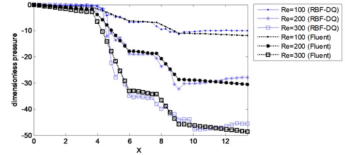
(b) 2D channel flow with two obstructions

(c) 2D channel flow with three obstructions

3.3. Result on flow characteristics

Table 4 shows the comparison of error between upwind local RBF-DQ method and CFD-Fluent method, it is seen that the numerical solutions converge for varying Reynolds numbers. The predicted velocity vectors for 2D channel flow with different obstructions are shown in Fig. 4a, b and c, respectively. The velocity vectors become crowded above the obstruction, indicating flow acceleration in the narrow section. The minimum velocity occurs just downstream of the obstruction, creating a dead zone. Subsequently the flow starts to develop and recover to its original profile along the channel. As $R e$ increases, the recirculation in this dead zone increases.

Table 4A comparison of error between RBF-DQ method and CFD-Fluent method

Flow type	$R e = 100$ $(a_{l} = 3, a_{r} = 2)$		$R e = 200$ $(a_{l} = 3, a_{r} = 2)$		$R e = 300$ $(a_{l} = 4, a_{r} = 2)$
Flow type	$μ$ (%)	$σ$ (%)	$μ$ (%)	$σ$ (%)	$μ$ (%)	$σ$ (%)
Channel flow with one obstruction	1.61	3.25	2.38	3.77	3.10	4.34
Channel flow with two obstructions	3.57	4.23	4.16	4.59	4.46	5.64
Channel flow with three obstructions	4.78	5.06	4.96	5.68	5.46	5.89

The predicted pressure distributions along the lower wall for channel flow with different obstructions are presented in Fig. 5 for both RBF-DQ and CFD-Fluent models. The two sets of results are in good agreement. The wall pressure decreases slowly from the channel entrance to the obstruction as the flow resistance. Then it drops rapidly on the obstruction due to the bigger velocity gradient on the obstruction. Subsequently the wall shear stress increases slowly as the flow recovers towards the outlet.

4. Conclusions

In this study, we have developed a novel method based on the upwind local RBF-DQ method for direction solution of the Navier–Stokes equations. We validated the proposed method by studying the classical flow situations, namely, the 2D channel flow with different obstructions. The predicted results are then compared with the well validated commercial code for the channel flow.

Numerical results show that the upwind local RBF-DQ method is well suited to solve irregular regions. Although the method has been developed in the context of two-dimensional problem, it can be extended to three-dimensional problem is fairly straightforward. It is hoped that the insights presented in this paper will help to spur more interest in and launch more investigations into the use of RBF-DQ method for the numerical flow simulation.

References

J. Monaghan A turbulence model for smoothed particle hydrodynamics. European Journal of Mechanics-B/Fluids, Vol. 30, 2011, p. 360-370.

Search CrossRef
K. Selim, A. Logg, M. G. Larson An adaptive finite element splitting method for the incompressible Navier–Stokes equations. Computer Methods in Applied Mechanics and Engineering, 2011.

Search CrossRef
N. Nguyen, J. Peraire, B. Cockburn An implicit high-order hybridizable discontinuous Galerkin method for the incompressible Navier–Stokes equations. Journal of Computational Physics, Vol. 230, 2011, p. 1147-1170.

Search CrossRef
P. Guan, S. Chi, J. Chen, T. Slawson, M. Roth Semi-Lagrangian reproducing kernel particle method for fragment-impact problems. International Journal of Impact Engineering, Vol. 38, 2011, p. 1033-1047.

Search CrossRef
J. Xu, S. Rajendran A partition-of-unity based ‘FE-Meshfree’QUAD4 element with radial-polynomial basis functions for static analyses. Computer Methods in Applied Mechanics and Engineering, Vol. 200, 2011, p. 3309-3323.

Search CrossRef
C. A. Duarte, J. T. Oden Hp clouds-an hp meshless method. Numerical methods for partial differential equations, Vol. 12, 1996, p. 673-706.

Search CrossRef
F. Perazzo, R. Löhner, L. Perez-Pozo Adaptive methodology for meshless finite point method. Advances in Engineering Software, Vol. 39, 2008, p. 156-166.

Search CrossRef
W. L. Nicomedes, R. C. Mesquita, F. J. S. Moreira The meshless local Petrov–Galerkin method in two-dimensional electromagnetic wave analysis. IEEE Transactions on Antennas and Propagation, Vol. 60, 2012, p. 1957-1968.

Search CrossRef
B. Ataie-Ashtiani, L. Farhadi A stable moving-particle semi-implicit method for free surface flows. Fluid Dynamics Research, Vol. 38, 2006, p. 241-256.

Search CrossRef
T. Liszka An interpolation method for an irregular net of nodes. International Journal for Numerical Methods in Engineering, Vol. 20, 2005, p. 1599-1612.

Search CrossRef
E. J. Kansa Multiquadrics–A scattered data approximation scheme with applications to computational fluid-dynamics–I surface approximations and partial derivative estimates. Computers & Mathematics with Applications, Vol. 19, 1990, p. 127-145.

Search CrossRef
E. J. Kansa Multiquadrics–A scattered data approximation scheme with applications to computational fluid-dynamics–II solutions to parabolic, hyperbolic and elliptic partial differential equations. Computers & Mathematics with Applications, Vol. 19, 1990, p. 147-161.

Search CrossRef
G. E. Fasshauer Solving partial differential equations by collocation with radial basis functions. Proceedings of Chamonix, Vanderbilt University Press, Nashville, TN, 1996, p. 1-8.

Search CrossRef
G. Demirkaya, C. Wafo Soh, O. Ilegbusi Direct solution of Navier–Stokes equations by radial basis functions. Applied Mathematical Modelling, Vol. 32, 2008, p. 1848-1858.

Search CrossRef
T. A. Driscoll, B. Fornberg Interpolation in the limit of increasingly flat radial basis functions. Computers & Mathematics with Applications, Vol. 43, 2002, p. 413-422.

Search CrossRef
Y. Hon, Z. Wu A quasi‐interpolation method for solving stiff ordinary differential equations. International Journal for Numerical Methods in Engineering, Vol. 48, 2000, p. 1187-1197.

Search CrossRef
W. Chen, M. Tanaka A meshless, integration-free, and boundary-only RBF technique. Computers & Mathematics with applications, Vol. 43, 2002, p. 379-391.

Search CrossRef
C. Chen, C. Brebbia The dual reciprocity method for Helmholtz-type operators. Boundary elements, Vol. 10, 1998, p. 495-504.

Search CrossRef
S. Xiang, G. Li, W. Zhang, M. Yang A meshless local radial point collocation method for free vibration analysis of laminated composite plates. Composite Structures, Vol. 93, 2011, p. 280-286.

Search CrossRef
W. Zongmin Hermite-Birkhoff interpolation of scattered data by radial basis functions. Approximation Theory and its Applications, Vol. 8, 1992, p. 1-10.

Search CrossRef
C. W. Bert, M. Malik Differential quadrature method in computational mechanics: a review. Applied Mechanics Reviews, Vol. 49, 1996.

Search CrossRef
C. Shu, H. Ding, H. Chen, T. Wang An upwind local RBF-DQ method for simulation of inviscid compressible flows. Computer Methods in Applied Mechanics and Engineering, Vol. 194, 2005, p. 2001-2017.

Search CrossRef
J. Sun, Z. Zhu Upwind local differential quadrature method for solving incompressible viscous flow. Computer Methods in Applied Mechanics and Engineering, Vol. 188, 2000, p. 495-504.

Search CrossRef
A. H. D. Cheng, M. Golberg, E. Kansa, G. Zammito Exponential convergence and H‐c multiquadric collocation method for partial differential equations. Numerical Methods for Partial Differential Equations, Vol. 19, 2003, p. 571-594.

Search CrossRef
M. D. Buhmann Radial basis functions: theory and implementations. Cambridge University Press, 2003.

Search CrossRef
M. Griebel, M. A. Schweitzer Meshfree methods for partial differential equations. Springer Verlag, 2003.

Search CrossRef
S. Patankar Numerical Heat Transfer and Fluid Flow. Hemisphere, Washington, DC, 1980, The FLUENT (trademark of FLUENT Inc.) fluid dynamics analysis package has been used in this study, 1980.

Search CrossRef
E. Divo, A. J. Kassab A meshless method for conjugate heat transfer problems. Engineering Analysis with Boundary Elements, Vol. 29, 2005, p. 136-149.

Search CrossRef
K. Madsen, H. B. Nielsen, J. Søndergaard Robust Subroutines for Non-Linear Optimization. IMM, Informatics and Mathematical Modelling, Technical University of Denmark, 2002.

Search CrossRef

About this article

Received

02 September 2013

Accepted

05 November 2013

Published

15 February 2014

Keywords

radial basis function-based differential quadrature method

upwind mechanism

Navier-Stokes equations

Acknowledgements

This research was supported by the Natural Science Foundation of China (No. 11302133) and Education Fund Item of Liaoning Province (No. L2013071). I am grateful to Dr. Tianzhi Yang for reading the manuscript and for helpful suggestions.

This is an open access article distributed under the Creative Commons Attribution License, which permits unrestricted use, distribution, and reproduction in any medium, provided the original work is properly cited.